Tracking Accuracy of a Feedback system

At this stage, we do not specify a particular controller. Instead, we analyze the steady-state error from the open-loop transfer function \(G(s)H(s)\).

Show code cell source Hide code cell source

from IPython.core.display import HTML
import numpy as np

import matplotlib.pyplot as plt
plt.rcParams.update({
    "text.usetex": True,
    "font.family": "serif",
    "font.size": 10,
})

from sympy import *
from sympy.plotting import plot

from mathprint import *

Show code cell source Hide code cell source

t = symbols('t', real=True)
s = symbols('s', complex=True)
a, b = symbols('a b', real=True, positive=True)
G, H, R, E, C, Ess = symbols('G H R E C E_ss', complex=True)
K = symbols("K", positive=True)

Define a system \(G(s)\) with a feedback \(H(s)\). The input is \(r(t)\) and the output is \(c(t)\).

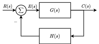
Define the error:

\(e(t) = r(t) - c(t)\)

and the steady state error:

\(e_{ss} = \lim\limits_{t \to \infty} e(t)\)

With final value theorem:

\(e_{ss} = \lim\limits_{s \to 0} sE(s)\)

eq1 = Eq(E, R - H*C)
eq2 = Eq(C, G*E)

sol = solve((eq1, eq2), (E, C))

mprint("E = ", latex(sol[E]))
mprint("C = ", latex(sol[C]))

\[\displaystyle E = \frac{R}{G H + 1}\]

\[\displaystyle C = \frac{G R}{G H + 1}\]

In classical control theory, steady-state error is commonly evaluated using three standard test inputs: the step input, the ramp input, and the parabolic input.

System Types

Define system type as the number of pure integrators in the open-loop transfer function \(G(s)H(s)\). The open-loop system is assumed to be stable with one real pole in LHP.

GH_type0 = K/(s + a)
GH_type1 = K/(s*(s + a))
GH_type2 = K/(s**2*(s + a))

mprint("GH_{type0} = ", latex(GH_type0))
mprint("GH_{type1} = ", latex(GH_type1))
mprint("GH_{type2} = ", latex(GH_type2))

\[\displaystyle GH_{type0} = \frac{K}{a + s}\]

\[\displaystyle GH_{type1} = \frac{K}{s \left(a + s\right)}\]

\[\displaystyle GH_{type2} = \frac{K}{s^{2} \left(a + s\right)}\]

Step Input

E_type0 = together(sol[E].subs(G*H, GH_type0).subs(R, 1/s))
ess_step_type0 = together(limit(s*E_type0, s, 0))

mprint("E_{type0}(s) = ", latex(E_type0))
mprint("e_{ss,type0} = ", latex(ess_step_type0))

\[\displaystyle E_{type0}(s) = \frac{a + s}{s \left(K + a + s\right)}\]

\[\displaystyle e_{ss,type0} = \frac{a}{K + a}\]

E_type1 = together(sol[E].subs(G*H, GH_type1).subs(R, 1/s))
ess_step_type1 = together(limit(s*E_type1, s, 0))

mprint("E_{type1}(s) = ", latex(E_type1))
mprint("e_{ss,type1} = ", latex(ess_step_type1))

\[\displaystyle E_{type1}(s) = \frac{a + s}{K + s \left(a + s\right)}\]

\[\displaystyle e_{ss,type1} = 0\]

E_type2 = together(sol[E].subs(G*H, GH_type2).subs(R, 1/s))
ess_step_type2 = together(limit(s*E_type2, s, 0))

mprint("E_{type2}(s) = ", latex(E_type2))
mprint("e_{ss,type2} = ", latex(ess_step_type2))

\[\displaystyle E_{type2}(s) = \frac{s \left(a + s\right)}{K + s^{2} \left(a + s\right)}\]

\[\displaystyle e_{ss,type2} = 0\]

Ramp Input

E_type0 = together(sol[E].subs(G*H, GH_type0).subs(R, 1/(s**2)))
ess_ramp_type0 = together(limit(s*E_type0, s, 0, dir="+"))

mprint("E_{type0}(s) = ", latex(E_type0))
mprint("e_{ss,type0} = ", latex(ess_ramp_type0))

\[\displaystyle E_{type0}(s) = \frac{a + s}{s^{2} \left(K + a + s\right)}\]

\[\displaystyle e_{ss,type0} = \infty\]

E_type1 = together(sol[E].subs(G*H, GH_type1).subs(R, 1/(s**2)))
ess_ramp_type1 = together(limit(s*E_type1, s, 0, dir="+"))

mprint("E_{type1}(s) = ", latex(E_type1))
mprint("e_{ss,type1} = ", latex(ess_ramp_type1))

\[\displaystyle E_{type1}(s) = \frac{a + s}{s \left(K + s \left(a + s\right)\right)}\]

\[\displaystyle e_{ss,type1} = \frac{a}{K}\]

E_type2 = together(sol[E].subs(G*H, GH_type2).subs(R, 1/(s**2)))
ess_ramp_type2 = together(limit(s*E_type2, s, 0, dir="+"))

mprint("E_{type2}(s) = ", latex(E_type2))
mprint("e_{ss,type2} = ", latex(ess_ramp_type2))

\[\displaystyle E_{type2}(s) = \frac{a + s}{K + s^{2} \left(a + s\right)}\]

\[\displaystyle e_{ss,type2} = 0\]

Parabolic Input

E_type0 = together(sol[E].subs(G*H, GH_type0).subs(R, 1/(s**3)))
ess_parabolic_type0 = together(limit(s*E_type0, s, 0))

mprint("E_{type0}(s) = ", latex(E_type0))
mprint("e_{ss,type0} = ", latex(ess_parabolic_type0))

\[\displaystyle E_{type0}(s) = \frac{a + s}{s^{3} \left(K + a + s\right)}\]

\[\displaystyle e_{ss,type0} = \infty\]

E_type1 = together(sol[E].subs(G*H, GH_type1).subs(R, 1/(s**3)))
ess_parabolic_type1 = together(limit(s*E_type1, s, 0))

mprint("E_{type1}(s) = ", latex(E_type1))
mprint("e_{ss,type1} = ", latex(ess_parabolic_type1))

\[\displaystyle E_{type1}(s) = \frac{a + s}{s^{2} \left(K + s \left(a + s\right)\right)}\]

\[\displaystyle e_{ss,type1} = \infty\]

E_type2 = together(sol[E].subs(G*H, GH_type2).subs(R, 1/(s**3)))
ess_parabolic_type2 = together(limit(s*E_type2, s, 0))

mprint("E_{type2}(s) = ", latex(E_type2))
mprint("e_{ss,type2} = ", latex(ess_parabolic_type2))

\[\displaystyle E_{type2}(s) = \frac{a + s}{s \left(K + s^{2} \left(a + s\right)\right)}\]

\[\displaystyle e_{ss,type2} = \frac{a}{K}\]

Summary

Show code cell source Hide code cell source

from pandas import DataFrame
from IPython.display import Markdown

def makelatex(args):
    return ["$\\Large {}$".format(latex(a)) for a in args]

legends = ["Step", "Ramp", "Parabolic"]
type0 = [ess_step_type0, ess_ramp_type0, ess_parabolic_type0]
type1 = [ess_step_type1, ess_ramp_type1,
        ess_parabolic_type1]
type2 = [ess_step_type2, ess_ramp_type2,
        ess_parabolic_type2]

dic = {'Input': legends, 
       'Type 0': makelatex(type0),
       'Type 1': makelatex(type1),
       'Type 2': makelatex(type2)}

df = DataFrame(dic)
Markdown(df.to_markdown(index=False))

Input	Type 0	Type 1	Type 2
Step	\(\Large \frac{a}{K + a}\)	\(\Large 0\)	\(\Large 0\)
Ramp	\(\Large \infty\)	\(\Large \frac{a}{K}\)	\(\Large 0\)
Parabolic	\(\Large \infty\)	\(\Large \infty\)	\(\Large \frac{a}{K}\)