The Bode Plots

Our goals:

• Draw the Bode plots with symbolic math.

• Explore the asymptotic Bode plots that is found in general control text books and express theses text-book steps into more generalized piecewise linear funtions.

Preparations

Show code cell source Hide code cell source

import numpy as np

from sympy import *
from sympy.physics.control.lti import TransferFunction

from mathprint import *

import matplotlib.pyplot as plt
plt.rcParams.update({
    "text.usetex": True,
    "font.family": "serif",
    "font.size": 10,
})

Define variables that we are going to use repetitively. We also need to define specific prpoperties of the variables.

t        = symbols('t'       , real=True)
s        = symbols('s'       , complex=True)
omega    = symbols('omega'   , positive=True)
a, b     = symbols('a b'     , real=True)
zeta     = symbols('zeta'    , positive=True)
omega_n  = symbols('omega_n' , positive=True)

Bode Plots with Symbolic Math

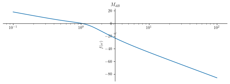
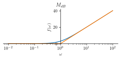
The Bode plots consist of two plots, the magnitude plot and the phase plot. To obtain these two plots, we substitute \(s=j \omega\) to the transfer function \(G(s)\) that we want to investigate.

Let us take the following transfer function as an example.

G = (0.5*s + 1.3) / (s**3 + 1.2*s**2 + 1.6*s)
mprint("G(s)=", latex(G))

\[\displaystyle G(s)=\frac{0.5 s + 1.3}{s^{3} + 1.2 s^{2} + 1.6 s}\]

By substituting \(s = j \omega\), we obtain:

Gjw = G.subs(s, I*omega)
mprint("G(j\\omega)=", latex(Gjw))

\[\displaystyle G(j\omega)=\frac{0.5 i \omega + 1.3}{- i \omega^{3} - 1.2 \omega^{2} + 1.6 i \omega}\]

Next, we extract the magnitude and the phase equations. The magnitude equation is \(M(\omega)\):

M = Abs(Gjw)
mprint("M=", latex(M))

Mdb = 20*log(M,10)
mprint("M_{dB} = ", latex(Mdb))

\[\displaystyle M=\frac{0.8125 \sqrt{0.14792899408284 \omega^{2} + 1}}{\sqrt{0.390625 \omega^{6} - 0.6875 \omega^{4} + \omega^{2}}}\]

\[\displaystyle M_{dB} = \frac{20 \log{\left(\frac{0.8125 \sqrt{0.14792899408284 \omega^{2} + 1}}{\sqrt{0.390625 \omega^{6} - 0.6875 \omega^{4} + \omega^{2}}} \right)}}{\log{\left(10 \right)}}\]

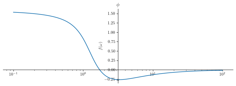
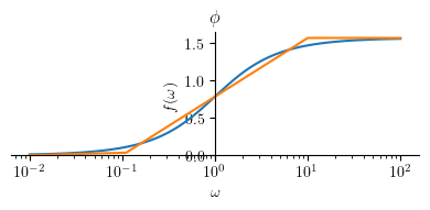
The phase equation is \(\phi(\omega)\):

Phi = simplify(atan(im(Gjw)/re(Gjw)))
mprint("\\phi = ", latex(Phi))

\[\displaystyle \phi = \operatorname{atan}{\left(\frac{2.08 - 0.7 \omega^{2}}{\omega \left(0.5 \omega^{2} + 0.76\right)} \right)}\]

Finally, we plot the two plots seperately.

mag = plot(Mdb, (omega, 0.1 , 100), size=(8, 3), show=False, title='$ M_{dB} $', xscale='log')
mag.show()

pha = plot(Phi, (omega, 0.1 , 100), size=(8, 3), title='$ \\phi $', show=False,  xscale='log')
pha.show()

In summary, these are the fundamental steps that we must do to plot the frequence response (Bode plot) of a system defined by a transfer function \(G(s)\):

• Do substitution: \(s = j \omega\) to \(G(s)\)

• Compute \(G( j \omega )\)

• The result is a complex function:

  • Extract the magnitude function: \( M = \big| G(j \omega) \big| \)

  • Convert the magnitude into dB: \( M_{dB} = 20 \log_{10} M \)

  • Extract the the phase function: \( \phi = \angle G(j \omega) \)

Asymptotic Bode Plots of Low-Order Transfer Functions

It is very easy to execute those steps by using a computer. On the other hand, when we simply want to sketch the Bode plot without using a computer, we can use the asymptotic method to draw the approximated version of the Bode plot.

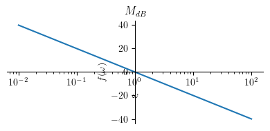
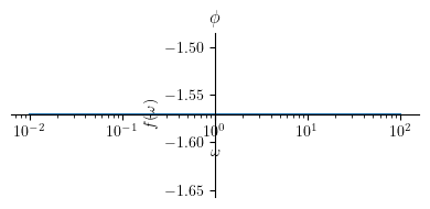
Case 1: A pole at the origin of the s-plane

Let us start by first defining the transfer function:

H1 = 1/s
mprint('H(s)=', latex(H1))

\[\displaystyle H(s)=\frac{1}{s}\]

After the substitution, we then obtain:

Hjw  = H1.subs(s, I*omega)
M1   = simplify(Abs(Hjw))
Mdb1 = simplify(20*log(M1, 10))
Phi1 = arg(Hjw)
mprintb("M  =", latex(M1))
mprintb("M_{dB} =", latex(Mdb1))
mprintb("\\phi =", latex(Phi1))

\[\displaystyle \boxed{M =\frac{1}{\omega}}\]

\[\displaystyle \boxed{M_{dB} =- \frac{20 \log{\left(\omega \right)}}{\log{\left(10 \right)}}}\]

\[\displaystyle \boxed{\phi =- \frac{\pi}{2}}\]

Magnitude plot:

Show code cell source Hide code cell source

title = '$ M_{dB} $'
p1 = plot(Mdb1, (omega, 0.01 , 100), size=(4, 2), title=title, show=True,  xscale='log')

Phase plot:

Show code cell source Hide code cell source

title = '$\\phi $'
p2 = plot(Phi1, (omega, 0.01 , 100), size=(4, 2), title=title, show=True,  xscale='log')

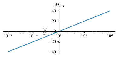
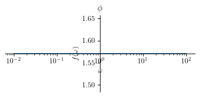
Case 2: A zero at the origin of the s-plane

Let us start by first defining the transfer function:

H2 = s
mprint('H(s)=', latex(H2))

\[\displaystyle H(s)=s\]

After the substitution, we then obtain:

Hjw  = H2.subs(s, I*omega)
M2   = simplify(Abs(Hjw))
Mdb2 = simplify(20 * log(M2, 10))
Phi2 = arg(Hjw)
mprintb("M  =", latex(M2))
mprintb("M_{dB} =", latex(Mdb2))
mprintb("\\phi =", latex(Phi2))

\[\displaystyle \boxed{M =\omega}\]

\[\displaystyle \boxed{M_{dB} =\frac{20 \log{\left(\omega \right)}}{\log{\left(10 \right)}}}\]

\[\displaystyle \boxed{\phi =\frac{\pi}{2}}\]

Magnitude plot:

Show code cell source Hide code cell source

title = '$M_{dB}$'
p1 = plot(Mdb2, (omega, 0.01 , 100), size=(4, 2), title=title, show=True,  xscale='log')

Phase plot:

Show code cell source Hide code cell source

title = '$\\phi $'
p2 = plot(Phi2, (omega, 0.01 , 100), size=(4, 2), title=title, show=True,  xscale='log')

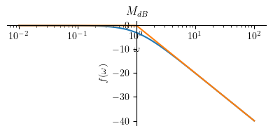
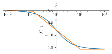
Case 3: A single real pole

Let us start by first defining the transfer function:

H3 = 1/(s+a)
mprint('H(s)=', latex(H3))

\[\displaystyle H(s)=\frac{1}{a + s}\]

After the substitution, we then obtain:

Hjw  = H3.subs(s, I*omega)
M3   = simplify(Abs(Hjw))
Mdb3 = simplify(20 * log(M3, 10))
Phi3 = arg(Hjw)
mprintb("M =", latex(M3))
mprintb("M_{dB} =", latex(Mdb3))
mprintb("\\phi =", latex(Phi3))

\[\displaystyle \boxed{M =\frac{1}{\sqrt{a^{2} + \omega^{2}}}}\]

\[\displaystyle \boxed{M_{dB} =- \frac{10 \log{\left(a^{2} + \omega^{2} \right)}}{\log{\left(10 \right)}}}\]

\[\displaystyle \boxed{\phi =\arg{\left(\frac{1}{a + i \omega} \right)}}\]

Now, let us plot the results for both the magnitude and the phase. To do this, we must first set a numerical value for \(a\). Let us set \(a=1\).

a_ = 1

Next, let us write down the approximated version of the plots, for the magnitude and the phase. What we do here is a bit based on observations.

Magnitude plot:

Mhatdb3 = Piecewise((-20 * log(a, 10),     omega <= a),
                    (-20 * log(omega, 10), True))
mprintb("\\hat{ M }_{dB} = ", latex(Mhatdb3))

\[\begin{split}\displaystyle \boxed{\hat{ M }_{dB} = \begin{cases} - \frac{20 \log{\left(a \right)}}{\log{\left(10 \right)}} & \text{for}\: a \geq \omega \\- \frac{20 \log{\left(\omega \right)}}{\log{\left(10 \right)}} & \text{otherwise} \end{cases}}\end{split}\]

Show code cell source Hide code cell source

title = '$M_{dB}$'
p1 = plot(Mdb3.subs(a, a_),    (omega, a_/100 , 100*a_), size=(4, 2), title=title, show=False,  xscale='log')
p2 = plot(Mhatdb3.subs(a, a_), (omega, a_/100 , 100*a_), show=False)
p1.append(p2[0])
p1.show()

Phase plot:

Phihat3 = Piecewise((0, omega <= 0.1*a),
                    (-pi/4 * log(omega/(0.1*a), 10) , omega < a*10), 
                    (-pi/2, True))
mprintb("\\hat{ \\phi }  = ", latex(simplify(Phihat3)))

\[\begin{split}\displaystyle \boxed{\hat{ \phi } = \begin{cases} 0 & \text{for}\: 0.1 a \geq 1.0 \omega \\- \frac{\pi \log{\left(\frac{10.0 \omega}{a} \right)}}{4 \log{\left(10 \right)}} & \text{for}\: \omega < 10 a \\- \frac{\pi}{2} & \text{otherwise} \end{cases}}\end{split}\]

Show code cell source Hide code cell source

title = '$ \\phi $'
p1 = plot(Phi3.subs(a, a_),    (omega, a_/100 , 100*a_), size=(4, 2), title=title, show=False,  xscale='log')
p2 = plot(Phihat3.subs(a, a_), (omega, a_/100 , 100*a_), show=False)
p1.append(p2[0])
p1.show()

Case 4: A single real zero

Let us start by first defining the transfer function:

H4 = s+a
mprint('H(s)=', latex(H4))

\[\displaystyle H(s)=a + s\]

After the substitution, we then obtain:

Hjw  = H4.subs(s, I*omega)
M4   = simplify(Abs(Hjw))
Mdb4 = simplify(20 * log(M4, 10))
Phi4 = arg(Hjw)
mprint("M  =", latex(M4))
mprint("M_{dB} =", latex(Mdb4))
mprint("\\phi =", latex(Phi4))

\[\displaystyle M =\sqrt{a^{2} + \omega^{2}}\]

\[\displaystyle M_{dB} =\frac{10 \log{\left(a^{2} + \omega^{2} \right)}}{\log{\left(10 \right)}}\]

\[\displaystyle \phi =\arg{\left(a + i \omega \right)}\]

Now, let us plot the results for both the magnitude and the phase. To do this, we must first set a numerical value for \(a\). Let us set \(a=1\).

Next, let us write down the approximated version of the plots, for both the magnitude and the phase. What we do here is a bit based on observations.

Magnitude plot:

Mhatdb4 = Piecewise((20 * log(a, 10), omega <= a),
                    (20 * log(omega, 10), True))
mprintb("\\hat{ M }_{dB} = ", latex(Mhatdb4))

\[\begin{split}\displaystyle \boxed{\hat{ M }_{dB} = \begin{cases} \frac{20 \log{\left(a \right)}}{\log{\left(10 \right)}} & \text{for}\: a \geq \omega \\\frac{20 \log{\left(\omega \right)}}{\log{\left(10 \right)}} & \text{otherwise} \end{cases}}\end{split}\]

Show code cell source Hide code cell source

title = '$M_{dB}$'
p1 = plot(Mdb4.subs(a, a_),    (omega, a_/100 , 100*a_), size=(4, 2), title=title, show=False,  xscale='log')
p2 = plot(Mhatdb4.subs(a, a_), (omega, a_/100 , 100*a_), show=False)
p1.append(p2[0])
p1.show()

Phase plot:

Phihat4 = Piecewise((0, omega <= 0.1*a),
                    (pi/4 * log(omega/(0.1*a), 10) , omega < a*10), 
                    (pi/2, True))
mprintb("\\hat{ \\phi } = ", latex(simplify(Phihat4)))

\[\begin{split}\displaystyle \boxed{\hat{ \phi } = \begin{cases} 0 & \text{for}\: 0.1 a \geq 1.0 \omega \\\frac{\pi \log{\left(\frac{10.0 \omega}{a} \right)}}{4 \log{\left(10 \right)}} & \text{for}\: \omega < 10 a \\\frac{\pi}{2} & \text{otherwise} \end{cases}}\end{split}\]

Show code cell source Hide code cell source

title = '$ \\phi $'
p1 = plot(Phi4.subs(a, a_),    (omega, a_/100 , 100*a_), size=(4, 2), title=title, show=False,  xscale='log')
p2 = plot(Phihat4.subs(a, a_), (omega, a_/100 , 100*a_), show=False)
p1.append(p2[0])
p1.show()

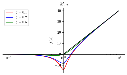
Case 5: Complex Conjugate Pole Pair

Let us start by first defining the transfer function:

H5 = 1 / (s**2 + 2*zeta*omega_n*s + omega_n**2)
mprint('H(s)=', latex(H5))

\[\displaystyle H(s)=\frac{1}{\omega_{n}^{2} + 2 \omega_{n} s \zeta + s^{2}}\]

By substituting \(s\) with \(j \omega\), we can obtain:

Hjw  = H5.subs(s, I*omega)
M5   = simplify(Abs(Hjw))
Mdb5 = expand_log(20 * log(M5, 10))
Phi5 = arg(Hjw)
mprint("M =", latex(M5))
mprint("M_{dB} =", latex(Mdb5))
mprint("\\phi =", latex(Phi5))

\[\displaystyle M =\frac{1}{\sqrt{\omega^{4} + 4 \omega^{2} \omega_{n}^{2} \zeta^{2} - 2 \omega^{2} \omega_{n}^{2} + \omega_{n}^{4}}}\]

\[\displaystyle M_{dB} =- \frac{10 \log{\left(\omega^{4} + 4 \omega^{2} \omega_{n}^{2} \zeta^{2} - 2 \omega^{2} \omega_{n}^{2} + \omega_{n}^{4} \right)}}{\log{\left(10 \right)}}\]

\[\displaystyle \phi =\arg{\left(\frac{1}{- \omega^{2} + 2 i \omega \omega_{n} \zeta + \omega_{n}^{2}} \right)}\]

Resonance peak:

• Complex conjugate pole pair occurs when \(\zeta < 1\).

• When \(\zeta < 1\), the system becomes underdamped and resonace peak appears in the magnitude plot.

• Resonance peak appears at \(\omega_p\) and its peak magnitude is \(M_p\).

omega_p5 = solve(Eq(diff(M5, omega), 0), omega)
mprintb("\\omega_p=", latex(omega_p5[0]))

\[\displaystyle \boxed{\omega_p=\omega_{n} \sqrt{1 - 2 \zeta^{2}}}\]

Mp5 = simplify(M5.subs(omega, omega_p5[0]))
Mdbp5 =simplify(Mdb5.subs(omega, omega_p5[0]))
mprintb("M_p = ", latex(Mp5))
mprintb("M_{p(dB)} = ", latex(Mdbp5))

\[\displaystyle \boxed{M_p = \frac{1}{2 \omega_{n}^{2} \zeta \sqrt{1 - \zeta^{2}}}}\]

\[\displaystyle \boxed{M_{p(dB)} = - \frac{10 \log{\left(- 4 \omega_{n}^{4} \zeta^{2} \left(\zeta^{2} - 1\right) \right)}}{\log{\left(10 \right)}}}\]

Now, let’s express the asymptotic Bode plot as piecewise functions. At the moment, we will do this by intuition.

Mhatdb5 = Piecewise((-40 * log(omega_n, 10), omega <= omega_n),
                    (-40 * log(omega, 10), omega > omega_n))
mprintb("\\hat{ M }_{dB} ( \\omega ) = ", latex(Mhatdb5))

\[\begin{split}\displaystyle \boxed{\hat{ M }_{dB} ( \omega ) = \begin{cases} - \frac{40 \log{\left(\omega_{n} \right)}}{\log{\left(10 \right)}} & \text{for}\: \omega \leq \omega_{n} \\- \frac{40 \log{\left(\omega \right)}}{\log{\left(10 \right)}} & \text{otherwise} \end{cases}}\end{split}\]

Magnitude plot:

For plotting, we need to define some numerical values for:

omega_n_ = 1
zeta_ = [0.1, 0.2, 0.5] # plot for several values

Show code cell source Hide code cell source

title = '$ M_{dB} $'
p1 = plot(Mdb5.subs(([omega_n, omega_n_],[zeta, zeta_[0]])),    (omega, omega_n_/10 , 10*omega_n_), line_color='r', size=(5, 3), title=title, show=False,  xscale='log', legend=True)
p2 = plot(Mdb5.subs(([omega_n, omega_n_],[zeta, zeta_[1]])),    (omega, omega_n_/10 , 10*omega_n_), line_color='b', show=False)
p3 = plot(Mdb5.subs(([omega_n, omega_n_],[zeta, zeta_[2]])),    (omega, omega_n_/10 , 10*omega_n_), line_color='g', show=False)
p4 = plot(Mhatdb5.subs(([omega_n, omega_n_],[zeta, zeta_[0]])), (omega, omega_n_/10 , 10*omega_n_), line_color='k', show=False)

p1[0].label = "$\\zeta=" + str(zeta_[0]) + "$"
p2[0].label = "$\\zeta=" + str(zeta_[1]) + "$"
p3[0].label = "$\\zeta=" + str(zeta_[2]) + "$"
p4[0].label = ""

p1.append(p2[0])
p1.append(p3[0])
p1.append(p4[0])

p1.show()

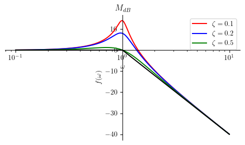
The general shape of the asymptotic magnitude plot is not affected by \(\zeta\).

We are not going to include the resonance peak for the asymptotic plots. However, we can still compute this peak value by using the equation expressed by \(M_{p(dB)}\):

print(Mdbp5.subs(([omega_n, omega_n_],[zeta, zeta_[0]])).evalf()) # for zeta[0]
print(Mdbp5.subs(([omega_n, omega_n_],[zeta, zeta_[1]])).evalf()) # for zeta[1]
print(Mdbp5.subs(([omega_n, omega_n_],[zeta, zeta_[2]])).evalf()) # for zeta[2]

14.0230481407449
8.13608784304507
1.24938736608300

Resonance peak happens at \(\omega = \omega_{p}\):

print(omega_p5[0].subs(([omega_n, omega_n_],[zeta, zeta_[0]])).evalf())

0.989949493661167

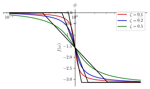
Phase plot:

Phihat5 = Piecewise((0, omega <= (omega_n / 10**zeta)),
                    (-pi/(2*zeta) * log(omega/(10**(-zeta)*omega_n), 10) , omega < (omega_n*10**zeta)), 
                    (-pi, True))
mprintb("\\hat{ \\phi } ( \\omega ) = ", latex(Phihat5))

\[\begin{split}\displaystyle \boxed{\hat{ \phi } ( \omega ) = \begin{cases} 0 & \text{for}\: \omega \leq 10^{- \zeta} \omega_{n} \\- \frac{\pi \log{\left(\frac{10^{\zeta} \omega}{\omega_{n}} \right)}}{2 \zeta \log{\left(10 \right)}} & \text{for}\: \omega < 10^{\zeta} \omega_{n} \\- \pi & \text{otherwise} \end{cases}}\end{split}\]

Show code cell source Hide code cell source

title = '$ \\phi $'
p1 = plot(Phi5.subs(([omega_n, omega_n_],[zeta, zeta_[0]])),    (omega, omega_n_/10 , 10*omega_n_), line_color='r', size=(5, 3), title=title, show=False,  xscale='log', legend=True)
p2 = plot(Phi5.subs(([omega_n, omega_n_],[zeta, zeta_[1]])),    (omega, omega_n_/10 , 10*omega_n_), line_color='b', show=False)
p3 = plot(Phi5.subs(([omega_n, omega_n_],[zeta, zeta_[2]])),    (omega, omega_n_/10 , 10*omega_n_), line_color='g', show=False)

p4 = plot(Phihat5.subs(([omega_n, omega_n_],[zeta, zeta_[0]])), (omega, omega_n_/10 , 10*omega_n_), line_color='k', show=False)
p5 = plot(Phihat5.subs(([omega_n, omega_n_],[zeta, zeta_[1]])), (omega, omega_n_/10 , 10*omega_n_), line_color='k', show=False)
p6 = plot(Phihat5.subs(([omega_n, omega_n_],[zeta, zeta_[2]])), (omega, omega_n_/10 , 10*omega_n_), line_color='k', show=False)


p1[0].label = "$\\zeta=" + str(zeta_[0]) + "$"
p2[0].label = "$\\zeta=" + str(zeta_[1]) + "$"
p3[0].label = "$\\zeta=" + str(zeta_[2]) + "$"
p4[0].label = ""
p5[0].label = ""
p6[0].label = ""

p1.append(p2[0])
p1.append(p3[0])
p1.append(p4[0])
p1.append(p5[0])
p1.append(p6[0])

p1.show()

Case 6: Complex Conjugate Zero Pair

Let us start by first defining the transfer function:

H6 = (s**2 + 2*zeta*omega_n*s + omega_n**2) 
mprint('H(s)=', latex(H6))

\[\displaystyle H(s)=\omega_{n}^{2} + 2 \omega_{n} s \zeta + s^{2}\]

Hjw  = H6.subs(s, I*omega)
M6   = simplify(Abs(Hjw))
Mdb6 = simplify(20 * log(M6, 10))
Phi6 = arg(Hjw)
mprint("M  =", latex(M6))
mprint("M_{dB}  =", latex(Mdb6))
mprint("\\phi  =", latex(Phi6))

\[\displaystyle M =\sqrt{\omega^{4} + 4 \omega^{2} \omega_{n}^{2} \zeta^{2} - 2 \omega^{2} \omega_{n}^{2} + \omega_{n}^{4}}\]

\[\displaystyle M_{dB} =\frac{10 \log{\left(\omega^{4} + 4 \omega^{2} \omega_{n}^{2} \zeta^{2} - 2 \omega^{2} \omega_{n}^{2} + \omega_{n}^{4} \right)}}{\log{\left(10 \right)}}\]

\[\displaystyle \phi =\arg{\left(- \omega^{2} + 2 i \omega \omega_{n} \zeta + \omega_{n}^{2} \right)}\]

Resonance peak:

Complex conjugate zero pair occurs when \(\zeta < 1\). Resonance peak appears in the Bode magnitude plot at \(\omega = \omega_n\). The magnitude at this resonance peak can be computed as:

omega_p6 = solve(Eq(diff(M6, omega), 0), omega)
mprintb("\\omega_p=", latex(omega_p6[0]))

\[\displaystyle \boxed{\omega_p=\omega_{n} \sqrt{1 - 2 \zeta^{2}}}\]

Mp6 = simplify(M6.subs(omega, omega_p6[0]))
Mdbp6 =simplify(Mdb6.subs(omega, omega_p6[0]))
mprintb("M_p = ", latex(Mp6))
mprintb("M_{p(dB)} = ", latex(Mdbp6))

\[\displaystyle \boxed{M_p = 2 \omega_{n}^{2} \zeta \sqrt{1 - \zeta^{2}}}\]

\[\displaystyle \boxed{M_{p(dB)} = \frac{10 \log{\left(4 \omega_{n}^{4} \zeta^{2} \left(1 - \zeta^{2}\right) \right)}}{\log{\left(10 \right)}}}\]

Magnitude plot:

We first present the piecewise logarithmic representation of the asymptotic Bode plot. After that, we present the plot for several diffrent values for \(\zeta\).

Mhatdb6 = Piecewise((40 * log(omega_n, 10), omega < omega_n),
                    (40 * log(omega, 10), omega >= omega_n))
mprintb("\\hat{ M } ( \\omega ) = ", latex(Mhatdb6))

\[\begin{split}\displaystyle \boxed{\hat{ M } ( \omega ) = \begin{cases} \frac{40 \log{\left(\omega_{n} \right)}}{\log{\left(10 \right)}} & \text{for}\: \omega < \omega_{n} \\\frac{40 \log{\left(\omega \right)}}{\log{\left(10 \right)}} & \text{otherwise} \end{cases}}\end{split}\]

Show code cell source Hide code cell source

title = '$ M_{dB} $'
p1 = plot(Mdb6.subs(([omega_n, omega_n_],[zeta, zeta_[0]])),    (omega, omega_n_/10 , 10*omega_n_), line_color='r', size=(5, 3), title=title, show=False,  xscale='log', legend=True)
p2 = plot(Mdb6.subs(([omega_n, omega_n_],[zeta, zeta_[1]])),    (omega, omega_n_/10 , 10*omega_n_), line_color='b', show=False)
p3 = plot(Mdb6.subs(([omega_n, omega_n_],[zeta, zeta_[2]])),    (omega, omega_n_/10 , 10*omega_n_), line_color='g', show=False)
p4 = plot(Mhatdb6.subs(([omega_n, omega_n_],[zeta, zeta_[0]])), (omega, omega_n_/10 , 10*omega_n_), line_color='k', show=False)

p1[0].label = "$\\zeta=" + str(zeta_[0]) + "$"
p2[0].label = "$\\zeta=" + str(zeta_[1]) + "$"
p3[0].label = "$\\zeta=" + str(zeta_[2]) + "$"
p4[0].label = ""

p1.append(p2[0])
p1.append(p3[0])
p1.append(p4[0])

p1.show()

The general shape of the asymptotic magnitude plot is not affected by \(\zeta\).

We are not going to include the resonance peak for the asymptotic plots. However, we can still compute this peak value by using the equation expressed by \(M_{p(dB)}\):

print(Mdbp6.subs(([omega_n, omega_n_],[zeta, zeta_[0]])).evalf()) # for zeta[0]
print(Mdbp6.subs(([omega_n, omega_n_],[zeta, zeta_[1]])).evalf()) # for zeta[1]
print(Mdbp6.subs(([omega_n, omega_n_],[zeta, zeta_[2]])).evalf()) # for zeta[2]

-14.0230481407449
-8.13608784304507
-1.24938736608300

Resonance peak happens at \(\omega = \omega_{p}\):

print(omega_p6[0].subs(([omega_n, omega_n_],[zeta, zeta_[0]])).evalf())

0.989949493661167

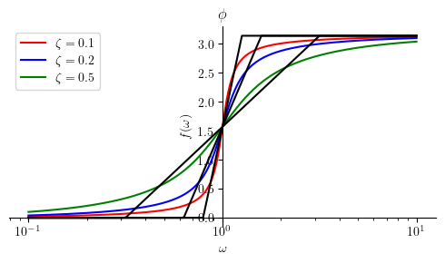
Phase plot:

Similar to the prevoius section, we first present the piecewise logarithmic representation of the asymptotic Bode plot. After that, we present the plot for several diffrent values for \(\zeta\).

Phihat6 = Piecewise((0, omega <= (omega_n / 10**zeta)),
                    (pi/(2*zeta) * log(omega/(10**(-zeta)*omega_n), 10) , omega < (omega_n*10**zeta)), 
                    (pi, True))
mprintb("\\hat{ \\phi } ( \\omega ) = ", latex(Phihat6))

\[\begin{split}\displaystyle \boxed{\hat{ \phi } ( \omega ) = \begin{cases} 0 & \text{for}\: \omega \leq 10^{- \zeta} \omega_{n} \\\frac{\pi \log{\left(\frac{10^{\zeta} \omega}{\omega_{n}} \right)}}{2 \zeta \log{\left(10 \right)}} & \text{for}\: \omega < 10^{\zeta} \omega_{n} \\\pi & \text{otherwise} \end{cases}}\end{split}\]

Show code cell source Hide code cell source

title = '$ \\phi $'
p1 = plot(Phi6.subs(([omega_n, omega_n_],[zeta, zeta_[0]])),    (omega, omega_n_/10 , 10*omega_n_), line_color='r', size=(5, 3), title=title, show=False,  xscale='log', legend=True)
p2 = plot(Phi6.subs(([omega_n, omega_n_],[zeta, zeta_[1]])),    (omega, omega_n_/10 , 10*omega_n_), line_color='b', show=False)
p3 = plot(Phi6.subs(([omega_n, omega_n_],[zeta, zeta_[2]])),    (omega, omega_n_/10 , 10*omega_n_), line_color='g', show=False)

p4 = plot(Phihat6.subs(([omega_n, omega_n_],[zeta, zeta_[0]])), (omega, omega_n_/10 , 10*omega_n_), line_color='k', show=False)
p5 = plot(Phihat6.subs(([omega_n, omega_n_],[zeta, zeta_[1]])), (omega, omega_n_/10 , 10*omega_n_), line_color='k', show=False)
p6 = plot(Phihat6.subs(([omega_n, omega_n_],[zeta, zeta_[2]])), (omega, omega_n_/10 , 10*omega_n_), line_color='k', show=False)

p1.append(p2[0])
p1.append(p3[0])
p1.append(p4[0])
p1.append(p5[0])
p1.append(p6[0])

p1[0].label = "$\\zeta=" + str(zeta_[0]) + "$"
p2[0].label = "$\\zeta=" + str(zeta_[1]) + "$"
p3[0].label = "$\\zeta=" + str(zeta_[2]) + "$"
p4[0].label = ""
p5[0].label = ""
p6[0].label = ""


p1.show()

Summary

Finally, let us summarize all boxed formulas.

Asymptotic Bode as piecewise functions

The following table shows piecewise approximations of a Bode plot.

Show code cell source Hide code cell source

from pandas import DataFrame
from IPython.display import Markdown

def makelatex(args):
    return ["${}$".format(latex(a)) for a in args]

Hs   = [H1, H2, H3, H4, H5, H6]
Mdbs = [Mdb1, Mdb2, Mhatdb3, Mhatdb4, Mhatdb5, Mhatdb6]
Phis = [Phi1, Phi2, Phihat3, Phihat4, Phihat5, Phihat6]

dic = {'$ H(s) $': makelatex(Hs), 
       '$ M_{dB} $': makelatex(Mdbs), 
       '$ \\phi $': makelatex(Phis)}

df = DataFrame(dic)
Markdown(df.to_markdown(index=False))

\( H(s) \)	\( M_{dB} \)	\( \phi \)
\(\frac{1}{s}\)	\(- \frac{20 \log{\left(\omega \right)}}{\log{\left(10 \right)}}\)	\(- \frac{\pi}{2}\)
\(s\)	\(\frac{20 \log{\left(\omega \right)}}{\log{\left(10 \right)}}\)	\(\frac{\pi}{2}\)
\(\frac{1}{a + s}\)	\(\begin{cases} - \frac{20 \log{\left(a \right)}}{\log{\left(10 \right)}} & \text{for}\: a \geq \omega \\- \frac{20 \log{\left(\omega \right)}}{\log{\left(10 \right)}} & \text{otherwise} \end{cases}\)	\(\begin{cases} 0 & \text{for}\: \omega \leq 0.1 a \\- \frac{\pi \log{\left(\frac{10.0 \omega}{a} \right)}}{4 \log{\left(10 \right)}} & \text{for}\: \omega < 10 a \\- \frac{\pi}{2} & \text{otherwise} \end{cases}\)
\(a + s\)	\(\begin{cases} \frac{20 \log{\left(a \right)}}{\log{\left(10 \right)}} & \text{for}\: a \geq \omega \\\frac{20 \log{\left(\omega \right)}}{\log{\left(10 \right)}} & \text{otherwise} \end{cases}\)	\(\begin{cases} 0 & \text{for}\: \omega \leq 0.1 a \\\frac{\pi \log{\left(\frac{10.0 \omega}{a} \right)}}{4 \log{\left(10 \right)}} & \text{for}\: \omega < 10 a \\\frac{\pi}{2} & \text{otherwise} \end{cases}\)
\(\frac{1}{\omega_{n}^{2} + 2 \omega_{n} s \zeta + s^{2}}\)	\(\begin{cases} - \frac{40 \log{\left(\omega_{n} \right)}}{\log{\left(10 \right)}} & \text{for}\: \omega \leq \omega_{n} \\- \frac{40 \log{\left(\omega \right)}}{\log{\left(10 \right)}} & \text{otherwise} \end{cases}\)	\(\begin{cases} 0 & \text{for}\: \omega \leq 10^{- \zeta} \omega_{n} \\- \frac{\pi \log{\left(\frac{10^{\zeta} \omega}{\omega_{n}} \right)}}{2 \zeta \log{\left(10 \right)}} & \text{for}\: \omega < 10^{\zeta} \omega_{n} \\- \pi & \text{otherwise} \end{cases}\)
\(\omega_{n}^{2} + 2 \omega_{n} s \zeta + s^{2}\)	\(\begin{cases} \frac{40 \log{\left(\omega_{n} \right)}}{\log{\left(10 \right)}} & \text{for}\: \omega < \omega_{n} \\\frac{40 \log{\left(\omega \right)}}{\log{\left(10 \right)}} & \text{otherwise} \end{cases}\)	\(\begin{cases} 0 & \text{for}\: \omega \leq 10^{- \zeta} \omega_{n} \\\frac{\pi \log{\left(\frac{10^{\zeta} \omega}{\omega_{n}} \right)}}{2 \zeta \log{\left(10 \right)}} & \text{for}\: \omega < 10^{\zeta} \omega_{n} \\\pi & \text{otherwise} \end{cases}\)

Resonance peaks

The following table summarizes when a resonance occurs and its peak value.

Show code cell source Hide code cell source

Hs   = [H5, H6]
wp   = [omega_p5[0], omega_p6[0]]
Mp   = [Mp5, Mp6]
Mpdb = [Mdbp5, Mdbp6]

dic = {'$H(s)$': makelatex(Hs), 
       '$ \\omega_p $': makelatex(wp), 
       '$ M_p $': makelatex(Mp),
       '$ M_{p(dB)} $': makelatex(Mpdb)}

df = DataFrame(dic)

Markdown(df.to_markdown(index=False))

\(H(s)\)	\( \omega_p \)	\( M_p \)	\( M_{p(dB)} \)
\(\frac{1}{\omega_{n}^{2} + 2 \omega_{n} s \zeta + s^{2}}\)	\(\omega_{n} \sqrt{1 - 2 \zeta^{2}}\)	\(\frac{1}{2 \omega_{n}^{2} \zeta \sqrt{1 - \zeta^{2}}}\)	\(- \frac{10 \log{\left(- 4 \omega_{n}^{4} \zeta^{2} \left(\zeta^{2} - 1\right) \right)}}{\log{\left(10 \right)}}\)
\(\omega_{n}^{2} + 2 \omega_{n} s \zeta + s^{2}\)	\(\omega_{n} \sqrt{1 - 2 \zeta^{2}}\)	\(2 \omega_{n}^{2} \zeta \sqrt{1 - \zeta^{2}}\)	\(\frac{10 \log{\left(4 \omega_{n}^{4} \zeta^{2} \left(1 - \zeta^{2}\right) \right)}}{\log{\left(10 \right)}}\)