
Digital High-Pass Filter#

In this section, we are going to do the following activities:

  • discretize a continuous-time high-pass filter by using bilinear transform (trapezoidal or Tustin) method

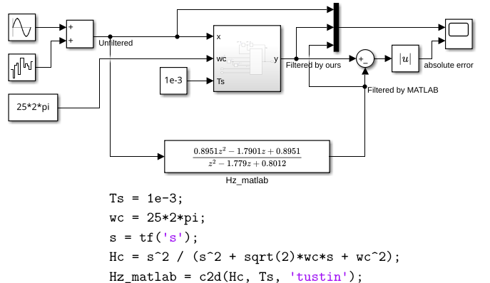
  • implement the discretized high-pass filter into MATLAB Simulink

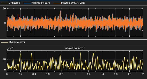
  • compare the results from the implemented discrete high-pass filter to the shipped discrete high-pass filter in MATLAB Simulink

Required Imports#

from IPython.core.display import HTML
from sympy import *
from mathprint import *
Ts, tau = symbols('T_s tau', positive=True)
s = symbols('s', complex=True)
z = symbols('z')
omega    = symbols('omega'   , positive=True)
wc = symbols('omega_c', positive=True)

x, y = symbols('x y')
x0, x1, x2, x3 = symbols('x_k x_{k-1} x_{k-2} x_{k-3}')
y0, y1, y2, y3 = symbols('y_k y_{k-1} y_{k-2} y_{k-3}')

First-Order High-Pass Filter#

The Complementary Form#

Transfer function of a first-order highpass filter as a complementary to a first-order lowpass filter(time-constant filter):

\[ H_{HP}(s) = 1 - H_{LP}\]
\[ H(s) = 1 - \frac{1} {\tau s+1} \]

where \(\tau\) is the filter time constant (in seconds).

Discretization with Bilinear Transformation

Next, we transform \(s\) into \(z\) by applying the following substitution.

\[ \frac{1}{s} \longleftarrow \frac{T_s}{2} \frac{z+1}{z-1} \]
H = 1 - 1 / (tau*s+1)
mprint('H=',latex(H))

H = H.subs(1/s, Ts/2 * (z+1)/(z-1))
mprint('H=',latex(H))
\[\displaystyle H=1 - \frac{1}{s \tau + 1}\]
\[\displaystyle H=1 - \frac{1}{1 + \frac{2 \tau \left(z - 1\right)}{T_{s} \left(z + 1\right)}}\]

Let us define \(x\) as the input to the filter and \(y\) as the output (filtered input).

eq = Eq(y, H * x)
mprint(latex(eq))

eq = simplify(eq)
mprint(latex(eq))

eq = Eq(numer(eq.rhs), expand(eq.lhs * denom(eq.rhs)))
mprint(latex(eq))

eq =expand(Eq(numer(eq.rhs)/z/Ts, eq.lhs * denom(eq.rhs)/z/Ts))
mprint(latex(eq))
\[\displaystyle y = x \left(1 - \frac{1}{1 + \frac{2 \tau \left(z - 1\right)}{T_{s} \left(z + 1\right)}}\right)\]
\[\displaystyle y = \frac{2 \tau x \left(z - 1\right)}{T_{s} \left(z + 1\right) + 2 \tau \left(z - 1\right)}\]
\[\displaystyle 2 \tau x \left(z - 1\right) = T_{s} y z + T_{s} y + 2 \tau y z - 2 \tau y\]
\[\displaystyle y + \frac{y}{z} + \frac{2 \tau y}{T_{s}} - \frac{2 \tau y}{T_{s} z} = \frac{2 \tau x}{T_{s}} - \frac{2 \tau x}{T_{s} z}\]

Apply the following substitutions:

  • \(y\) becomes \(y_{k}\)

  • \(y/z\) becomes \(y_{k-1}\)

  • \(x\) becomes \(x_{k}\)

  • \(x/z\) becomes \(x_{k-1}\)

eq = eq.subs(x/z**3, x3).subs(x/z**2, x2).subs(x/z, x1).subs(x, x0).subs(y/z**3, y3).subs(y/z**2, y2).subs(y/z, y1).subs(y, y0)
mprint("\\small ", latex(eq))
\[\displaystyle \small y_{k} + y_{k-1} + \frac{2 \tau y_{k}}{T_{s}} - \frac{2 \tau y_{k-1}}{T_{s}} = \frac{2 \tau x_{k}}{T_{s}} - \frac{2 \tau x_{k-1}}{T_{s}}\]

Finally, by grouping the variables, we obtain:

eq = Eq(collect(eq.rhs, [2,tau/Ts, x0, x1, x2, x3]), collect(eq.lhs, [y0, y1, y2, y3]) )
mprintb("\\small ", latex(eq))
\[\displaystyle \boxed{\small \frac{2 \tau x_{k}}{T_{s}} - \frac{2 \tau x_{k-1}}{T_{s}} = y_{k} \left(1 + \frac{2 \tau}{T_{s}}\right) + y_{k-1} \left(1 - \frac{2 \tau}{T_{s}}\right)}\]

Second Order High-Pass Butterworth Filter#

The Complementary Form#

Transfer function of a second order highpass filter as a complementary to a second-order lowpass filter (Butterworth):

\[ H_{HP}(s) = 1 - H_{LP}\]
\[ H(s) = 1 - \frac{\omega_{c}^{2}}{\omega_{c}^{2} + \sqrt{2} \omega_{c} s + s^{2}} \]

where \(\omega_c\) is the filter cut-off frequency (in Hz).

Discretization with Bilinear Transformation

Similiar to the previous section, here we also transform \(s\) into \(z\) by applying the following substitution.

\[ \frac{1}{s} \longleftarrow \frac{T_s}{2} \frac{z+1}{z-1} \]
H = 1 - wc**2 / (wc**2+sqrt(2)*s*wc+s**2)
mprint('H=',latex(H))

H = simplify(1 - wc**2 / (wc**2+sqrt(2)*s*wc+s**2))
mprint('H=',latex(H))

H = simplify(H.subs(1/s, Ts/2 * (z+1)/(z-1)))
mprint('H=',latex(H))
\[\displaystyle H=- \frac{\omega_{c}^{2}}{\omega_{c}^{2} + \sqrt{2} \omega_{c} s + s^{2}} + 1\]
\[\displaystyle H=\frac{s \left(\sqrt{2} \omega_{c} + s\right)}{\omega_{c}^{2} + \sqrt{2} \omega_{c} s + s^{2}}\]
\[\displaystyle H=\frac{2 \left(z - 1\right) \left(\sqrt{2} T_{s} \omega_{c} \left(z + 1\right) + 2 z - 2\right)}{T_{s}^{2} \omega_{c}^{2} \left(z + 1\right)^{2} + 2 \sqrt{2} T_{s} \omega_{c} \left(z - 1\right) \left(z + 1\right) + 4 \left(z - 1\right)^{2}}\]

Let us define \(x\) as the input to the filter and \(y\) as the output (filtered input).

eq = Eq(y, H * x)
mprint(latex(eq))

eq = simplify(eq)
mprint(latex(eq))

eq = Eq(numer(eq.rhs), expand(eq.lhs * denom(eq.rhs)))
mprint(latex(eq))

eq =expand(Eq(numer(eq.rhs)/z**2/Ts**2/wc**2, eq.lhs * denom(eq.rhs)/z**2/Ts**2/wc**2))
mprint(latex(eq))
\[\displaystyle y = \frac{2 x \left(z - 1\right) \left(\sqrt{2} T_{s} \omega_{c} \left(z + 1\right) + 2 z - 2\right)}{T_{s}^{2} \omega_{c}^{2} \left(z + 1\right)^{2} + 2 \sqrt{2} T_{s} \omega_{c} \left(z - 1\right) \left(z + 1\right) + 4 \left(z - 1\right)^{2}}\]
\[\displaystyle 2 x \left(z - 1\right) \left(\sqrt{2} T_{s} \omega_{c} \left(z + 1\right) + 2 z - 2\right) = T_{s}^{2} \omega_{c}^{2} y z^{2} + 2 T_{s}^{2} \omega_{c}^{2} y z + T_{s}^{2} \omega_{c}^{2} y + 2 \sqrt{2} T_{s} \omega_{c} y z^{2} - 2 \sqrt{2} T_{s} \omega_{c} y + 4 y z^{2} - 8 y z + 4 y\]
\[\displaystyle y + \frac{2 y}{z} + \frac{y}{z^{2}} + \frac{2 \sqrt{2} y}{T_{s} \omega_{c}} - \frac{2 \sqrt{2} y}{T_{s} \omega_{c} z^{2}} + \frac{4 y}{T_{s}^{2} \omega_{c}^{2}} - \frac{8 y}{T_{s}^{2} \omega_{c}^{2} z} + \frac{4 y}{T_{s}^{2} \omega_{c}^{2} z^{2}} = \frac{2 \sqrt{2} x}{T_{s} \omega_{c}} - \frac{2 \sqrt{2} x}{T_{s} \omega_{c} z^{2}} + \frac{4 x}{T_{s}^{2} \omega_{c}^{2}} - \frac{8 x}{T_{s}^{2} \omega_{c}^{2} z} + \frac{4 x}{T_{s}^{2} \omega_{c}^{2} z^{2}}\]

Apply the following substitutions:

  • \(y\) becomes \(y_{k}\)

  • \(y/z\) becomes \(y_{k-1}\)

  • \(y/z^2\) becomes \(y_{k-2}\)

  • \(x\) becomes \(x_{k}\)

  • \(x/z\) becomes \(x_{k-1}\)

  • \(x/z^2\) becomes \(x_{k-2}\)

eq = eq.subs(x/z**3, x3).subs(x/z**2, x2).subs(x/z, x1).subs(x, x0).subs(y/z**3, y3).subs(y/z**2, y2).subs(y/z, y1).subs(y, y0)
mprint(latex(eq))
\[\displaystyle y_{k} + 2 y_{k-1} + y_{k-2} + \frac{2 \sqrt{2} y_{k}}{T_{s} \omega_{c}} - \frac{2 \sqrt{2} y_{k-2}}{T_{s} \omega_{c}} + \frac{4 y_{k}}{T_{s}^{2} \omega_{c}^{2}} - \frac{8 y_{k-1}}{T_{s}^{2} \omega_{c}^{2}} + \frac{4 y_{k-2}}{T_{s}^{2} \omega_{c}^{2}} = \frac{2 \sqrt{2} x_{k}}{T_{s} \omega_{c}} - \frac{2 \sqrt{2} x_{k-2}}{T_{s} \omega_{c}} + \frac{4 x_{k}}{T_{s}^{2} \omega_{c}^{2}} - \frac{8 x_{k-1}}{T_{s}^{2} \omega_{c}^{2}} + \frac{4 x_{k-2}}{T_{s}^{2} \omega_{c}^{2}}\]

Finally, by grouping the variables, we obtain:

eq = Eq(collect(eq.rhs, [x0, x1, x2, x3]), collect(eq.lhs, [y0, y1, y2, y3]) )
mprintb(latex(eq))
\[\displaystyle \boxed{x_{k} \left(\frac{2 \sqrt{2}}{T_{s} \omega_{c}} + \frac{4}{T_{s}^{2} \omega_{c}^{2}}\right) + x_{k-2} \left(- \frac{2 \sqrt{2}}{T_{s} \omega_{c}} + \frac{4}{T_{s}^{2} \omega_{c}^{2}}\right) - \frac{8 x_{k-1}}{T_{s}^{2} \omega_{c}^{2}} = y_{k} \left(1 + \frac{2 \sqrt{2}}{T_{s} \omega_{c}} + \frac{4}{T_{s}^{2} \omega_{c}^{2}}\right) + y_{k-1} \left(2 - \frac{8}{T_{s}^{2} \omega_{c}^{2}}\right) + y_{k-2} \left(1 - \frac{2 \sqrt{2}}{T_{s} \omega_{c}} + \frac{4}{T_{s}^{2} \omega_{c}^{2}}\right)}\]

However, the complementary form does NOT have +40 dB/decade at \(\omega=\omega_c\). We will show this through these steps:

  • Substitute \(j\omega\) to \(s\) in \(H(s)\) and convert it to dB. We name is as \(M(j\omega)\).

  • Calculate \(S=\frac{dM}{d\omega}\)

These steps will give us the slope in db/(rad/s).

H = simplify(1 - wc**2 / (wc**2+sqrt(2)*s*wc+s**2))
Hjw = H.subs(s, I*omega)

M = 20*log(abs(Hjw))/log(10)
mprint('M(j\\omega)=', latex(M))

dM = simplify(diff(M, omega))
mprint('S(\\omega)=\\frac{dM(\\omega)}{d\\omega}=', latex(dM))
\[\displaystyle M(j\omega)=\frac{20 \log{\left(\frac{\omega \sqrt{\omega^{2} + 2 \omega_{c}^{2}}}{\sqrt{\omega^{4} + \omega_{c}^{4}}} \right)}}{\log{\left(10 \right)}}\]
\[\displaystyle S(\omega)=\frac{dM(\omega)}{d\omega}=\frac{40 \omega_{c}^{2} \left(- \omega^{4} + \omega^{2} \omega_{c}^{2} + \omega_{c}^{4}\right)}{\omega \left(\omega^{6} + 2 \omega^{4} \omega_{c}^{2} + \omega^{2} \omega_{c}^{4} + 2 \omega_{c}^{6}\right) \log{\left(10 \right)}}\]

However, the unit here is dB/(rad/s), not dB/decade. To obtain dB/decade:

Sdb = simplify(omega * log(10) * dM)
mprint("S_{dB}(\\omega)=", latex(Sdb))
\[\displaystyle S_{dB}(\omega)=\frac{40 \omega_{c}^{2} \left(- \omega^{4} + \omega^{2} \omega_{c}^{2} + \omega_{c}^{4}\right)}{\omega^{6} + 2 \omega^{4} \omega_{c}^{2} + \omega^{2} \omega_{c}^{4} + 2 \omega_{c}^{6}}\]

Let us take \(\omega_c=1\) and plot the slope for arbitrary \(\omega\).

Hide code cell source
Sdb_wc1 = simplify(Sdb.subs(wc, 1))

mprint(
    r'S_{\mathrm{dB}}(\omega)\big|_{\omega_c=1}=',
    latex(Sdb_wc1)
)

p = plot(
    Sdb_wc1,
    (omega, 0.1, 100),
    size=(5, 2),
    show=False,
    title=r'$S_{\mathrm{dB}}(\omega),\quad \omega_c=1$',
    xlabel=r'$\omega$',
    ylabel=r'dB/decade',
    xscale='log'
)

p.show()
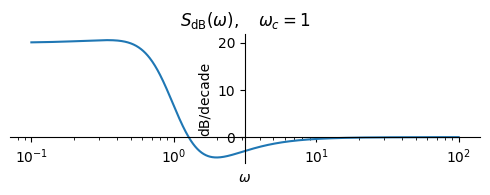
\[\displaystyle S_{\mathrm{dB}}(\omega)\big|_{\omega_c=1}=\frac{40 \left(- \omega^{4} + \omega^{2} + 1\right)}{\omega^{6} + 2 \omega^{4} + \omega^{2} + 2}\]
_images/c90acde96016f1d1840978a987d41673ddc1bc34c29a0d709a45949a4e21f382.png
Sdb_wc = simplify(Sdb.subs(omega, wc))
Sdb_wc
\[\displaystyle \frac{20}{3}\]

Thus, it is only about 6.7 dB / decade! We can assure this by checking maximum an minimum possible slopes, which is 0 dB / decade and 20 db / decade, respectively.

Sdb_low = simplify(limit(Sdb, omega, 0, dir='+'))
Sdb_high = simplify(limit(Sdb, omega, oo))

mprint(
    r'\lim_{\omega\to0}S_{\mathrm{dB}}(\omega)=',
    latex(Sdb_low)
)

mprint(
    r'\lim_{\omega\to\infty}S_{\mathrm{dB}}(\omega)=',
    latex(Sdb_high)
)
\[\displaystyle \lim_{\omega\to0}S_{\mathrm{dB}}(\omega)=20\]
\[\displaystyle \lim_{\omega\to\infty}S_{\mathrm{dB}}(\omega)=0\]

The complementary form has an asymptotic low-frequency slope of only +20 dB/decade, rather than the +40 dB/decade of a conventional second-order HPF. At the cutoff, its local slope is approximately +6.67 dB/decade.

Standard Form#

Since the complementary form only gives us 6.7dB / decade, while for a second order filter our target is 40 dB / decade, we must modify the filter equation slightly.

Infact, this is the standard form of a secon-dorder Butterworth highpass filter.

H = s**2 / (wc**2+sqrt(2)*s*wc+s**2)
mprintb('H=',latex(H))
\[\displaystyle \boxed{H=\frac{s^{2}}{\omega_{c}^{2} + \sqrt{2} \omega_{c} s + s^{2}}}\]
H = simplify(H.subs(1/s, Ts/2 * (z+1)/(z-1)))
mprint('H=',latex(H))
\[\displaystyle H=\frac{4 \left(z - 1\right)^{2}}{T_{s}^{2} \omega_{c}^{2} \left(z + 1\right)^{2} + 2 \sqrt{2} T_{s} \omega_{c} \left(z - 1\right) \left(z + 1\right) + 4 \left(z - 1\right)^{2}}\]
eq = Eq(y, H * x)
mprint(latex(eq))

eq = simplify(eq)
mprint(latex(eq))

eq = Eq(numer(eq.rhs), expand(eq.lhs * denom(eq.rhs)))
mprint(latex(eq))

eq =expand(Eq(numer(eq.rhs)/z**2/Ts**2/wc**2, eq.lhs * denom(eq.rhs)/z**2/Ts**2/wc**2))
mprint(latex(eq))
\[\displaystyle y = \frac{4 x \left(z - 1\right)^{2}}{T_{s}^{2} \omega_{c}^{2} \left(z + 1\right)^{2} + 2 \sqrt{2} T_{s} \omega_{c} \left(z - 1\right) \left(z + 1\right) + 4 \left(z - 1\right)^{2}}\]
\[\displaystyle 4 x \left(z - 1\right)^{2} = T_{s}^{2} \omega_{c}^{2} y z^{2} + 2 T_{s}^{2} \omega_{c}^{2} y z + T_{s}^{2} \omega_{c}^{2} y + 2 \sqrt{2} T_{s} \omega_{c} y z^{2} - 2 \sqrt{2} T_{s} \omega_{c} y + 4 y z^{2} - 8 y z + 4 y\]
\[\displaystyle y + \frac{2 y}{z} + \frac{y}{z^{2}} + \frac{2 \sqrt{2} y}{T_{s} \omega_{c}} - \frac{2 \sqrt{2} y}{T_{s} \omega_{c} z^{2}} + \frac{4 y}{T_{s}^{2} \omega_{c}^{2}} - \frac{8 y}{T_{s}^{2} \omega_{c}^{2} z} + \frac{4 y}{T_{s}^{2} \omega_{c}^{2} z^{2}} = \frac{4 x}{T_{s}^{2} \omega_{c}^{2}} - \frac{8 x}{T_{s}^{2} \omega_{c}^{2} z} + \frac{4 x}{T_{s}^{2} \omega_{c}^{2} z^{2}}\]
eq = eq.subs(x/z**3, x3).subs(x/z**2, x2).subs(x/z, x1).subs(x, x0).subs(y/z**3, y3).subs(y/z**2, y2).subs(y/z, y1).subs(y, y0)
mprint(latex(eq))
\[\displaystyle y_{k} + 2 y_{k-1} + y_{k-2} + \frac{2 \sqrt{2} y_{k}}{T_{s} \omega_{c}} - \frac{2 \sqrt{2} y_{k-2}}{T_{s} \omega_{c}} + \frac{4 y_{k}}{T_{s}^{2} \omega_{c}^{2}} - \frac{8 y_{k-1}}{T_{s}^{2} \omega_{c}^{2}} + \frac{4 y_{k-2}}{T_{s}^{2} \omega_{c}^{2}} = \frac{4 x_{k}}{T_{s}^{2} \omega_{c}^{2}} - \frac{8 x_{k-1}}{T_{s}^{2} \omega_{c}^{2}} + \frac{4 x_{k-2}}{T_{s}^{2} \omega_{c}^{2}}\]
eq = Eq(collect(eq.rhs, [x0, x1, x2, x3]), collect(eq.lhs, [y0, y1, y2, y3]) )
mprintb(latex(eq))
\[\displaystyle \boxed{\frac{4 x_{k}}{T_{s}^{2} \omega_{c}^{2}} - \frac{8 x_{k-1}}{T_{s}^{2} \omega_{c}^{2}} + \frac{4 x_{k-2}}{T_{s}^{2} \omega_{c}^{2}} = y_{k} \left(1 + \frac{2 \sqrt{2}}{T_{s} \omega_{c}} + \frac{4}{T_{s}^{2} \omega_{c}^{2}}\right) + y_{k-1} \left(2 - \frac{8}{T_{s}^{2} \omega_{c}^{2}}\right) + y_{k-2} \left(1 - \frac{2 \sqrt{2}}{T_{s} \omega_{c}} + \frac{4}{T_{s}^{2} \omega_{c}^{2}}\right)}\]