First-Order Systems

Required imports

from IPython.core.display import HTML
import numpy as np

import matplotlib.pyplot as plt
plt.rcParams.update({
    "text.usetex": True,
    "font.family": "Helvetica",
    "font.size": 10,
})

from sympy import *
from sympy.plotting import plot
from sympy.abc import x, y

from mathprint import *

Preparations

Define variables that we are going to use repetitively: \(s, t, \tau\). We also need to define specific prpoperties of the variables.

t   = symbols('t', real=True)
s   = symbols('s', complex=True)
tau = symbols('tau', real=True)

The original laplace transformation functions are a little too long. We will simplify the laplace and the inverse laplace transformation functions, as follows.

• laplace_transform(f, t, s, noconds=True) as laplace(f)

• inverse_laplace_transform(F, s, t) as ilapalce(F)

def laplace(f):
    F = laplace_transform(f, t, s, noconds=True)
    return F

def ilaplace(F):
    f = inverse_laplace_transform(F, s, t)
    return f

Special functions in SymPy

We will use these two special functions very often:

• \(\delta(t)\) is an impulse function or a Dirac Delta function

• \(\theta(t)\) is a step function or a Heaviside function

We can find more information about these functions here.

First-order system equation

A first-order system:

G = 1 / (tau*s + 1)
mprint('G(s)=\\frac{C(s)}{R(s)}=', latex(G))

\[\displaystyle G(s)=\frac{C(s)}{R(s)}=\frac{1}{s \tau + 1}\]

Here \(R(s)\) and \(C(s)\) are the input and output functions in \(s\)-domain, respectively. In time-domain, they become \(r(t)\) and \(c(t)\), respectively. The first order coefficient ( \(\tau\) ) is better known as the time constant.

Unit-impulse response

What we do here:

• define the input, which is a unit impulse function (Dirac Delta function)

r = DiracDelta(t)
mprint('r(t)=', latex(r))

\[\displaystyle r(t)=\delta\left(t\right)\]

• compute its Laplace form

R = laplace(r)
mprint('R(s)=', latex(R))

\[\displaystyle R(s)=1\]

• apply the input to the sytem and obtain the output

C = G*R
mprint('C(s)=', latex(C))

\[\displaystyle C(s)=\frac{1}{s \tau + 1}\]

• compute the inverse Laplace of the output

c = ilaplace(C)
mprint('c(t)=', latex(c))

\[\displaystyle c(t)=\frac{e^{- \frac{t}{\tau}} \theta\left(t\right)}{\tau}\]

For plotting the response, let us set \(\tau = 1\).

tau_ = 1
c1 = c.subs(tau, tau_)

p1 = plot(c1, (t, 0 , 7), ylim=[-0.5, 2], size=(4, 2.5), ylabel='$c(t)$', show=False, legend=True)
p2 = plot(-1/tau_**2*t + 1/tau_, (t, -1 , 7), show=False, legend=True)
p1[0].label = '$c(t)='+latex(c1)+'$'
p2[0].label = "gradient at $t=0$, $\\dot{c}(0)=-1$"
p1.append(p2[0])

p1.show() 

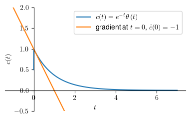
Two interesting informations that we can extract from the response plot above are:

• output value at \(t=0\) or \(\lim_{t \to 0} c(t)\)

limit(c, t, 0) # c(0)

\[\displaystyle \frac{1}{\tau}\]

• output gradient at \(t=0\) or \(\lim_{t \to 0}\frac{\mathtt{d}c}{\mathtt{d}t}\)

limit(diff(c, t), t, 0) # output gradient at t = 0

\[\displaystyle - \frac{1}{\tau^{2}}\]

Thus we can summarize, for unit-impulse output \(c(t)\):
$\(c(0) = \frac{1}{\tau}\)\( and \)\(\dot{c}(0) = -\frac{1}{\tau^2}\)$

Unit-step response

What we do here:

• define the input, which is a unit step function (Heaviside function)

t   = symbols('t', real=True, positive=True)

r = Heaviside(t)
mprint('r(t)=', latex(r))

\[\displaystyle r(t)=1\]

• compute its Laplace form

R = laplace(r)
mprint('R(s)=', latex(R))

\[\displaystyle R(s)=\frac{1}{s}\]

• apply the input to the sytem and obtain the output

C = G*R
mprint('C(s)=', latex(C))

\[\displaystyle C(s)=\frac{1}{s \left(s \tau + 1\right)}\]

• compute the inverse Laplace of the output

c = ilaplace(C)
mprint('c(t)=', latex(c))

\[\displaystyle c(t)=1 - e^{- \frac{t}{\tau}}\]

For plotting, let us set \(\tau = 1\).

tau_ = 1
c1 = collect(c.subs(tau, tau_), Heaviside(t))
mprint("c(t)=", latex(c1))

\[\displaystyle c(t)=1 - e^{- t}\]

tend = 6
p1 = plot(c1,                   (t,  0,   tend), ylim=[-0.2, 1.1], size=(4, 2.5), ylabel='$c(t)$', show=False)
p2 = plot_implicit(Eq(t, tau_), (t, -0.1, tend), line_color='r',show=False)  # vertical line at t = tau
p3 = plot(c1.subs(t, tau_),     (t, -0.3, tend), line_color='r', show=False) # horizontal line at c(tau)
p4 = plot(tau_*t,               (t, -0.3, tend), line_color='k', show=False) # gradient at t = 0
p1.append(p2[0])
p1.append(p3[0])
p1.append(p4[0])
p1.show()

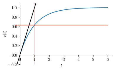
The figure above shows that at \(t = \tau\), \(c(\tau)\) is at \(63.21 \%\) of \(c_{ss}\)

• output value at \(t=\tau\) or \(c(\tau)\)

c1.subs(t,tau) # c(t = tau)

\[\displaystyle 1 - e^{- \tau}\]

• output gradient at \(t=0\) or \(\lim_{t \to 0} \frac{\mathtt{d}c}{\mathtt{d}t}\)

limit(diff(c, t), t, 0).evalf() # gradient at t = 0

\[\displaystyle \frac{1}{\tau}\]

Unit-ramp response

What we do here:

• define the input, which is a unit ramp function

r = t * Heaviside(t)
mprint('r(t)=', latex(r))

\[\displaystyle r(t)=t\]

• compute its Laplace form

R = laplace(r)
mprint('R(s)=', latex(R))

\[\displaystyle R(s)=\frac{1}{s^{2}}\]

• apply the input to the sytem and obtain the output

C = G*R
mprint('C(s)=', latex(C))

\[\displaystyle C(s)=\frac{1}{s^{2} \left(s \tau + 1\right)}\]

• compute the inverse Laplace of the output

c = collect(ilaplace(C), Heaviside(t))
mprint('c(t)=', latex(c))

\[\displaystyle c(t)=t - \tau + \tau e^{- \frac{t}{\tau}}\]

For plotting, let us set \(\tau = 1\).

tau_ = 1
c1 = collect(c.subs(tau, tau_), Heaviside(t))
mprint("c(t)=", latex(c1))

\[\displaystyle c(t)=t - 1 + e^{- t}\]

tend = 5
p1 = plot(c1, (t, 0, tend), ylim=[-0, 5], size=(2.5, 2.5), show=False, legend=True)
p2 = plot(r,  (t, 0, tend), line_color='r', show=False, legend=True)  
p1[0].label = '$r(t)$'
p2[0].label = '$c(t)$'
p1.append(p2[0])
p1.show()

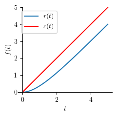
As we can see from the response plot above, there is a constant difference between the input and the output (vertical distance between red line and blue line). This constant difference can ba expressed as:

\[\Delta = \lim_{s \to 0} s\big(R(s)-C(s) \big) = \lim_{s \to 0} s \big(R(s)-GR(s) \big) = \lim_{s \to 0} sR(s) \big(1-G(s) \big) \]

delta = limit(s*laplace(r) * (1 - G), s, 0)
mprint('\\Delta=', latex(delta))

\[\displaystyle \Delta=\tau\]