Block Diagram

Block Diagram#

Series, Parallel and Feedback#

from sympy import symbols, prod,simplify, Eq, latex, solve, solveset

import matplotlib.pyplot as plt
plt.rcParams.update({
    "text.usetex": True,
    "font.family": "serif",
    "font.size": 10,
})

from mathprint import *

series(...) = Series connection: multiply transfer functions in cascade.
parallels(...) = Parallel connection: sum transfer functions connected in parallel.
negative_feedbacks(...) = Negative feedback: compute \(G/(1 + GH)\) for one or more feedback paths.
positive_feedback(...) = Positive feedback: compute \(G/(1 - GH)\) for one or more feedback paths.

def series(*argv):
    return prod(argv)

def parallels(*argv):
    return sum(argv)

def negative_feedbacks(G, *argv):
    ret = G
    for k in range(len(argv)):
        ret = ret / (1 + ret * argv[k])

    return ret

def positive_feedbacks(G, *argv):
    ret = G
    for k in range(len(argv)):
        ret = ret / (1 - ret * argv[k])
    
    return ret

Example 1#

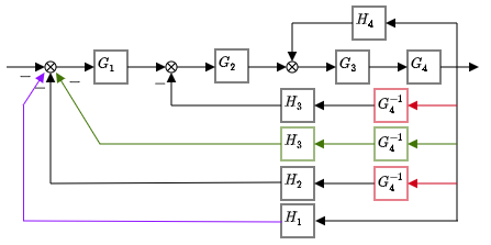
Simplify the following block diagram:

Our first step is to modify the block diagram such that it contains ony three connection configurations:

serial connections
parallel connections
feedback connections (positive or negative)

The next figure presents the modified block diagram that is composed only by those three connections.

M1 = series(G3, G4)
M2 = positive_feedbacks(M1, H4)
M3 = series(M2, G2)
M4 = negative_feedbacks(M3, H3/G4)
M5 = series(M4, G1)
G = negative_feedbacks(M5, H3/G4, H2/G4, H1)

Or we can combine them into one line of codes:

G = negative_feedbacks(series(negative_feedbacks(series(positive_feedbacks(series(G3, G4), H4), G2), H3/G4), G1), H3/G4, H2/G4, H1)

G1, G2, G3, G4, H1, H2, H3, H4 = symbols('G1 G2 G3 G4 H1 H2 H3 H4')

G = negative_feedbacks(series(negative_feedbacks(series(positive_feedbacks(series(G3, G4), H4), G2), H3/G4), G1), H3/G4, H2/G4, H1);
display(simplify(G))

\[\displaystyle \frac{G_{1} G_{2} G_{3} G_{4}}{G_{1} G_{2} G_{3} G_{4} H_{1} + G_{1} G_{2} G_{3} H_{2} + G_{1} G_{2} G_{3} H_{3} + G_{2} G_{3} H_{3} - G_{3} G_{4} H_{4} + 1}\]

Example 2#

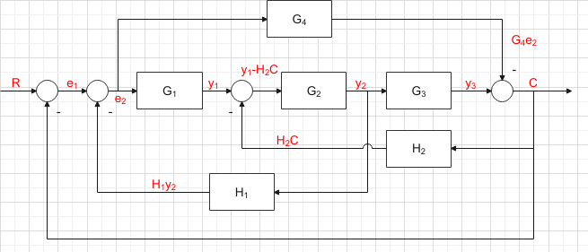
This problem is very difficult to solve with graphical method. Instead, we will use general algebra to solve the problem with SymPy.

There are at least 6 new intermediate variables: \(e_1\), \(e_2\), \(y_1\), \(y_2\), \(y_3\) and \(C\).
We need to setup at least 6 equations (see the red labels).
Solve those equations for all intermediate variables.

G1, G2, G3, G4   = symbols('G1 G2 G3 G4')
E, R, C = symbols('E R C')
e1, e2, y1, y2, y3 = symbols('e1 e2 y1 y2 y3')
s = symbols('s')

eq1 = Eq(R-C, e1)
eq2 = Eq(e1-H1*y2, e2)
eq3 = Eq(G1*e2, y1)
eq4 = Eq(G2*(y1-H2*C), y2)
eq5 = Eq(G3*y2, y3)
eq6 = Eq(y3-G4*e2, C)


mprint(latex(eq1))
mprint(latex(eq2)) 
mprint(latex(eq3))
mprint(latex(eq4))
mprint(latex(eq5))
mprint(latex(eq6))

\[\displaystyle - C + R = e_{1}\]

\[\displaystyle - H_{1} y_{2} + e_{1} = e_{2}\]

\[\displaystyle G_{1} e_{2} = y_{1}\]

\[\displaystyle G_{2} \left(- C H_{2} + y_{1}\right) = y_{2}\]

\[\displaystyle G_{3} y_{2} = y_{3}\]

\[\displaystyle - G_{4} e_{2} + y_{3} = C\]

Solve for the new intermediate variables:

ans = solve((eq1, eq2, eq3, eq4, eq5, eq6),  (C, e1, e2, y1, y2, y3))
for k in ans.keys():
    mprint(latex(k), '=', latex(ans[k]))

\[\displaystyle C=\frac{G_{1} G_{2} G_{3} R - G_{4} R}{G_{1} G_{2} G_{3} + G_{1} G_{2} H_{1} + G_{2} G_{3} H_{2} + G_{2} G_{4} H_{1} H_{2} - G_{4} + 1}\]

\[\displaystyle e_{1}=\frac{G_{1} G_{2} H_{1} R + G_{2} G_{3} H_{2} R + G_{2} G_{4} H_{1} H_{2} R + R}{G_{1} G_{2} G_{3} + G_{1} G_{2} H_{1} + G_{2} G_{3} H_{2} + G_{2} G_{4} H_{1} H_{2} - G_{4} + 1}\]

\[\displaystyle e_{2}=\frac{G_{2} G_{3} H_{2} R + R}{G_{1} G_{2} G_{3} + G_{1} G_{2} H_{1} + G_{2} G_{3} H_{2} + G_{2} G_{4} H_{1} H_{2} - G_{4} + 1}\]

\[\displaystyle y_{1}=\frac{G_{1} G_{2} G_{3} H_{2} R + G_{1} R}{G_{1} G_{2} G_{3} + G_{1} G_{2} H_{1} + G_{2} G_{3} H_{2} + G_{2} G_{4} H_{1} H_{2} - G_{4} + 1}\]

\[\displaystyle y_{2}=\frac{G_{1} G_{2} R + G_{2} G_{4} H_{2} R}{G_{1} G_{2} G_{3} + G_{1} G_{2} H_{1} + G_{2} G_{3} H_{2} + G_{2} G_{4} H_{1} H_{2} - G_{4} + 1}\]

\[\displaystyle y_{3}=\frac{G_{1} G_{2} G_{3} R + G_{2} G_{3} G_{4} H_{2} R}{G_{1} G_{2} G_{3} + G_{1} G_{2} H_{1} + G_{2} G_{3} H_{2} + G_{2} G_{4} H_{1} H_{2} - G_{4} + 1}\]

Now we take \(C = \dots\) and divide it by \(R\) to obtain \(C/R\):

tf = simplify(ans[C]/R)
mprintb("\\frac{C}{R} =", latex(tf))

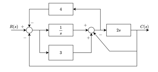
\[\displaystyle \boxed{\frac{C}{R} =\frac{G_{1} G_{2} G_{3} - G_{4}}{G_{1} G_{2} G_{3} + G_{1} G_{2} H_{1} + G_{2} G_{3} H_{2} + G_{2} G_{4} H_{1} H_{2} - G_{4} + 1}}\]

Example 3#

e1, y1, y2, y3, y4 = symbols('e1 y1 y2 y3 y4')
s = symbols('s')

eq1 = Eq(R-C-y1, e1)
eq2 = Eq(e1/s, y2)
eq3 = Eq(3*e1,y3)
eq4 = Eq(y2+y3-C, y4)
eq5 = Eq(4*y4, y1)
eq6 = Eq(y4*2*s, C)


mprint(latex(eq1))
mprint(latex(eq2)) 
mprint(latex(eq3))
mprint(latex(eq4))
mprint(latex(eq5))
mprint(latex(eq6))

\[\displaystyle - C + R - y_{1} = e_{1}\]

\[\displaystyle \frac{e_{1}}{s} = y_{2}\]

\[\displaystyle 3 e_{1} = y_{3}\]

\[\displaystyle - C + y_{2} + y_{3} = y_{4}\]

\[\displaystyle 4 y_{4} = y_{1}\]

\[\displaystyle 2 s y_{4} = C\]

ans = solve((eq1, eq2, eq3, eq4, eq5, eq6),  (C, e1, y1, y2, y3, y4))
for k in ans.keys():
    mprint(latex(k), '=', latex(ans[k]))

\[\displaystyle C=\frac{6 R s^{2} + 2 R s}{8 s^{2} + 15 s + 4}\]

\[\displaystyle e_{1}=\frac{2 R s^{2} + R s}{8 s^{2} + 15 s + 4}\]

\[\displaystyle y_{1}=\frac{12 R s + 4 R}{8 s^{2} + 15 s + 4}\]

\[\displaystyle y_{2}=\frac{2 R s + R}{8 s^{2} + 15 s + 4}\]

\[\displaystyle y_{3}=\frac{6 R s^{2} + 3 R s}{8 s^{2} + 15 s + 4}\]

\[\displaystyle y_{4}=\frac{3 R s + R}{8 s^{2} + 15 s + 4}\]

G = simplify(ans[C]/R)
mprintb("\\frac{C}{R} =", latex(G))

\[\displaystyle \boxed{\frac{C}{R} =\frac{2 s \left(3 s + 1\right)}{8 s^{2} + 15 s + 4}}\]

We can also try the graphical method by first converting the diagram into the following:

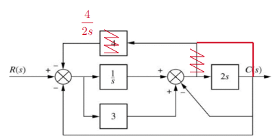
G = simplify(negative_feedbacks(series(parallels(1/s, 3), negative_feedbacks(2*s, 1)), 4/(2*s), 1))
mprintb("\\frac{C}{R} =", latex(G))