System Modeling: Flyball Governor

Preparations

from IPython.display import HTML
import numpy as np
import base64


import matplotlib.pyplot as plt
plt.rcParams.update({
    "text.usetex": True,
    "font.family": "Helvetica",
    "font.size": 10,
})

from sympy import *

from mathprint import *

# https://stackoverflow.com/questions/49145059/how-to-change-printed-representation-of-functions-derivative-in-sympy
latexReplaceRules = {
    # r'{\left(t \right)}':r' ',
    r'\frac{d}{d t}':r'\dot',
    r'\frac{d^{2}}{d t^{2}}':r'\ddot',
}

def latexNew(expr,**kwargs):
    retStr = latex(expr,**kwargs)
    for _,__ in latexReplaceRules.items():
        retStr = retStr.replace(_,__)
    return retStr


init_printing(use_unicode=False)
init_printing(latex_printer=latexNew)


def display_gif(fn):
    b64 = base64.b64encode(open(fn,'rb').read()).decode('ascii');
    display(HTML(f'<img src="data:image/gif;base64,{b64}" />'));

Declare the necessary symbols:

t = symbols('t', real=True)
theta1 = Function('theta1')
theta2 = Function('theta2')
tau    = symbols('tau', real=True)
J, m, l, d, g, b1, b2 = symbols('J m l d g b1 b2', real=True, nonnegative=True)

Kinetic energy

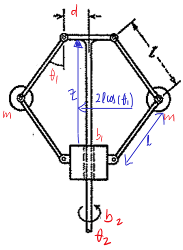
Let us describe the two motions that contribute to kinetic energy:

• upward-downward rotations around \(\theta_1\) \(\rightarrow T_1\)

• planar continous rotations around \(\theta_2\) \(\rightarrow T_2\)

Note that we use parallel axis theorem to compute the get the correct momen of inertia about the given rotation axis.

T1 = simplify( 2*1/2*(J+m*l**2)*diff(theta1(t) ,t)**2 )
T2 = simplify( 2*1/2*(J+m*(l*sin(theta1(t))+d)**2)*diff(theta2(t) ,t)**2 )

mprint('T_1=' + latexNew(T1))
mprint('T_2=' + latexNew(T2))

\[\displaystyle T_1=1.0 \left(J + l^{2} m\right) \left(\dot \theta_{1}{\left(t \right)}\right)^{2}\]

\[\displaystyle T_2=1.0 \left(J + m \left(d + l \sin{\left(\theta_{1}{\left(t \right)} \right)}\right)^{2}\right) \left(\dot \theta_{2}{\left(t \right)}\right)^{2}\]

Potential energy

V = 2*m*g*l*(1-cos(theta1(t)))

mprint('V=' + latexNew(V))

\[\displaystyle V=2 g l m \left(1 - \cos{\left(\theta_{1}{\left(t \right)} \right)}\right)\]

Dissipassion

We introudce two damping elements that cause energy lost:

• \(R_1\): dissipation by the linear bushing moving along the vertical rod.

• \(R_2\): dissipation by the rotating vertical rod.

z    = l-l*cos(theta1(t))
zdot = diff(z, t)

R1 = 1/2*b1*zdot**2
R2 = 1/2*b2*diff(theta2(t))**2

mprint('R_1=' + latexNew(R1))
mprint('R_2=' + latexNew(R2))

\[\displaystyle R_1=0.5 b_{1} l^{2} \sin^{2}{\left(\theta_{1}{\left(t \right)} \right)} \left(\dot \theta_{1}{\left(t \right)}\right)^{2}\]

\[\displaystyle R_2=0.5 b_{2} \left(\dot \theta_{2}{\left(t \right)}\right)^{2}\]

Euler–Lagrange equations

Now, we shall derive the Euler-Lagrange euqations step by step.

T = T1 + T2  # Total kinetic energy
L = T  - V   # The Lagrangian

dL_dTh = Matrix([diff(L, theta1(t)), diff(L, theta2(t))])

mprint('\\frac{dL}{d\\theta}=' + latexNew(dL_dTh))

\[\begin{split}\displaystyle \frac{dL}{d\theta}=\left[\begin{matrix}- 2 g l m \sin{\left(\theta_{1}{\left(t \right)} \right)} + 2.0 l m \left(d + l \sin{\left(\theta_{1}{\left(t \right)} \right)}\right) \cos{\left(\theta_{1}{\left(t \right)} \right)} \left(\dot \theta_{2}{\left(t \right)}\right)^{2}\\0\end{matrix}\right]\end{split}\]

dL_dThdot = simplify(Matrix([diff(L, diff(theta1(t), t)), diff(L, diff(theta2(t), t))]))

mprint('\\frac{dL}{d\\dot{\\theta}}=' + latexNew(dL_dThdot) )

\[\begin{split}\displaystyle \frac{dL}{d\dot{\theta}}=\left[\begin{matrix}2.0 \left(J + l^{2} m\right) \dot \theta_{1}{\left(t \right)}\\2.0 \left(J + m \left(d + l \sin{\left(\theta_{1}{\left(t \right)} \right)}\right)^{2}\right) \dot \theta_{2}{\left(t \right)}\end{matrix}\right]\end{split}\]

dR1_dThdot = simplify(Matrix([diff(R1, diff(theta1(t), t)), diff(R1, diff(theta2(t), t))]))

mprint('\\frac{dR_1}{d\\dot{\\theta}}=' + latexNew(dR1_dThdot) )

\[\begin{split}\displaystyle \frac{dR_1}{d\dot{\theta}}=\left[\begin{matrix}1.0 b_{1} l^{2} \sin^{2}{\left(\theta_{1}{\left(t \right)} \right)} \dot \theta_{1}{\left(t \right)}\\0\end{matrix}\right]\end{split}\]

dR2_dThdot = simplify(Matrix([diff(R2, diff(theta1(t), t)), diff(R2, diff(theta2(t), t))]))

mprint('\\frac{dR_2}{d\\dot{\\theta}}=' + latexNew(dR2_dThdot) )

\[\begin{split}\displaystyle \frac{dR_2}{d\dot{\theta}}=\left[\begin{matrix}0\\1.0 b_{2} \dot \theta_{2}{\left(t \right)}\end{matrix}\right]\end{split}\]

dL_dThdot_dt = simplify(Matrix([diff(diff(L, diff(theta1(t), t)),t) , diff(diff(L, diff(theta2(t), t)), t)]))
mprint('\\frac{dL}{d\\dot{\\theta} dt}=' + latexNew(dL_dThdot_dt) )

\[\begin{split}\displaystyle \frac{dL}{d\dot{\theta} dt}=\left[\begin{matrix}2.0 \left(J + l^{2} m\right) \ddot \theta_{1}{\left(t \right)}\\4.0 l m \left(d + l \sin{\left(\theta_{1}{\left(t \right)} \right)}\right) \cos{\left(\theta_{1}{\left(t \right)} \right)} \dot \theta_{1}{\left(t \right)} \dot \theta_{2}{\left(t \right)} + 2.0 \left(J + m \left(d + l \sin{\left(\theta_{1}{\left(t \right)} \right)}\right)^{2}\right) \ddot \theta_{2}{\left(t \right)}\end{matrix}\right]\end{split}\]

eq = simplify(dL_dThdot_dt - dL_dTh + dR1_dThdot + dR2_dThdot)

mprint('\\frac{dL}{d\\dot{\\theta} dt} - \\frac{dL}{d\\theta} + \\frac{dR_1}{d\\dot{\\theta}} + \\frac{dL}{d\\dot{\\theta} dt}=' + latexNew(eq) )

\[\begin{split}\displaystyle \frac{dL}{d\dot{\theta} dt} - \frac{dL}{d\theta} + \frac{dR_1}{d\dot{\theta}} + \frac{dL}{d\dot{\theta} dt}=\left[\begin{matrix}1.0 b_{1} l^{2} \sin^{2}{\left(\theta_{1}{\left(t \right)} \right)} \dot \theta_{1}{\left(t \right)} + 2 g l m \sin{\left(\theta_{1}{\left(t \right)} \right)} - 2.0 l m \left(d + l \sin{\left(\theta_{1}{\left(t \right)} \right)}\right) \cos{\left(\theta_{1}{\left(t \right)} \right)} \left(\dot \theta_{2}{\left(t \right)}\right)^{2} + 2.0 \left(J + l^{2} m\right) \ddot \theta_{1}{\left(t \right)}\\1.0 b_{2} \dot \theta_{2}{\left(t \right)} + 4.0 l m \left(d + l \sin{\left(\theta_{1}{\left(t \right)} \right)}\right) \cos{\left(\theta_{1}{\left(t \right)} \right)} \dot \theta_{1}{\left(t \right)} \dot \theta_{2}{\left(t \right)} + 2.0 \left(J + m \left(d + l \sin{\left(\theta_{1}{\left(t \right)} \right)}\right)^{2}\right) \ddot \theta_{2}{\left(t \right)}\end{matrix}\right]\end{split}\]

Equation of motions

By rewriting the Euler-Lagrange equations, we can then express the system’s equation of motions.

eqs = Eq(eq, Matrix([0 , tau]))

odes = solve(eqs, [diff(theta1(t), t, t), diff(theta2(t), t, t)])

ode1 = simplify(odes[diff(theta1(t), t, t)])
mprintb(" \\ddot{\\theta_1}(t) = ", latexNew(ode1))

\[\displaystyle \boxed{ \ddot{\theta_1}(t) = \frac{0.5 l \left(- b_{1} l \sin^{2}{\left(\theta_{1}{\left(t \right)} \right)} \dot \theta_{1}{\left(t \right)} + 2.0 d m \cos{\left(\theta_{1}{\left(t \right)} \right)} \left(\dot \theta_{2}{\left(t \right)}\right)^{2} - 2.0 g m \sin{\left(\theta_{1}{\left(t \right)} \right)} + 1.0 l m \sin{\left(2 \theta_{1}{\left(t \right)} \right)} \left(\dot \theta_{2}{\left(t \right)}\right)^{2}\right)}{J + l^{2} m}}\]

ode2 = simplify(odes[diff(theta2(t), t, t)])
mprintb(" \\ddot{\\theta_1}(t) = ", latexNew(ode2))

\[\displaystyle \boxed{ \ddot{\theta_1}(t) = \frac{- b_{2} \dot \theta_{2}{\left(t \right)} - 4.0 d l m \cos{\left(\theta_{1}{\left(t \right)} \right)} \dot \theta_{1}{\left(t \right)} \dot \theta_{2}{\left(t \right)} - 2.0 l^{2} m \sin{\left(2 \theta_{1}{\left(t \right)} \right)} \dot \theta_{1}{\left(t \right)} \dot \theta_{2}{\left(t \right)} + \tau}{2.0 J + 2.0 d^{2} m + 4.0 d l m \sin{\left(\theta_{1}{\left(t \right)} \right)} + 2.0 l^{2} m \sin^{2}{\left(\theta_{1}{\left(t \right)} \right)}}}\]

Numerical model

For demostration purposes, we will set some arbitrary numerical values to the parameters such that we can simulate the system.

We also need to define how we are going to actuate the system. The ideal input to the system is the torque: \( \tau(t) \). However, we can make the demonstration simpler by ignoring the second equation (ode2). This is possible if we assume we can apply instantaneous rotation (\( \dot{\theta}_2 \)) to the base of the device. Hence, in thise case we are only interested with how \( \dot{\theta}_2 \) afffects \( \theta_1 \) and \( \dot{\theta}_1 \).

m_ = 0.1
J_ = 0.01
l_ = 0.2
g_ = 9.8

b1_ = 5
b2_ = 0.1
d_ = 0.02
RPM_ = 100*0.10472 #converting RPM to rad/s

ode1n = simplify(ode1.subs(([m,  m_],
                            [b1, b1_],
                            [b2, b2_],
                            [J,  J_],
                            [l, l_],
                            [d, d_],
                            [g, g_])))
mprintb(" \\ddot{\\theta_1}(t) = ", latexNew(ode1n))

\[\displaystyle \boxed{ \ddot{\theta_1}(t) = - 7.14285714285714 \sin^{2}{\left(\theta_{1}{\left(t \right)} \right)} \dot \theta_{1}{\left(t \right)} - 14.0 \sin{\left(\theta_{1}{\left(t \right)} \right)} + 0.142857142857143 \sin{\left(2 \theta_{1}{\left(t \right)} \right)} \left(\dot \theta_{2}{\left(t \right)}\right)^{2} + 0.0285714285714286 \cos{\left(\theta_{1}{\left(t \right)} \right)} \left(\dot \theta_{2}{\left(t \right)}\right)^{2}}\]

ode2n = simplify(ode2.subs(([m,  m_],
                            [b1, b1_],
                            [b2, b2_],
                            [J,  J_],
                            [l, l_],
                            [d, d_],
                            [g, g_],
                            [tau, 0])))
mprintb(" \\ddot{\\theta_2}(t) = ", latexNew(ode2n))

\[\displaystyle \boxed{ \ddot{\theta_2}(t) = - \frac{\left(0.008 \sin{\left(2 \theta_{1}{\left(t \right)} \right)} \dot \theta_{1}{\left(t \right)} + 0.0016 \cos{\left(\theta_{1}{\left(t \right)} \right)} \dot \theta_{1}{\left(t \right)} + 0.1\right) \dot \theta_{2}{\left(t \right)}}{0.008 \sin^{2}{\left(\theta_{1}{\left(t \right)} \right)} + 0.0016 \sin{\left(\theta_{1}{\left(t \right)} \right)} + 0.02008}}\]

Numerical solutions

After plugging all parameters into the model, we can now solve the model numerically and obtain the motions as the results. To do this, we use the ODE solver that can be found in scipy.integrate. Also, we must put the model into its state-space form. The ODE solver takes the model only in a state-space form.

import scipy.integrate
import matplotlib.pyplot as plt

Complete state-space model

Let us introduce some new variables to descrive the system’s states: \(y=[y_0, y_1, y_2, y_3]\), where:

• \( y_0 = \theta_1 \)

• \( y_1 = \dot{\theta}_1 \)

• \( y_2 = \theta_2 \)

• \( y_3 = \dot{\theta}_2 \)

Hence, we also have: \( \dot{y}=[\dot{y}_0, \dot{y}_1, \dot{y}_2, \dot{y}_3] \), where:

• \( \dot{y}_0 = \dot{\theta_1} \)

• \( \dot{y}_1 = \ddot{\theta}_1 \)

• \( \dot{y}_2 = \dot{\theta_2} \)

• \( \dot{y}_3 = \ddot{\theta}_2 \)

# y[0] --> theta1
# y[1] --> theta1d
# y[2] --> theta2
# y[3] --> theta2d
y = symbols( 'y:4' )

ode1n_ = simplify(ode1n.subs(([diff(theta1(t), t), y[1]],
                              [diff(theta2(t), t), y[3]],
                              [theta1(t), y[0]],
                              [theta2(t), y[2]])))

ode2n_ = simplify(ode2n.subs(([diff(theta1(t), t), y[1]],
                              [diff(theta2(t), t), y[3]],
                              [theta1(t), y[0]],
                              [theta2(t), y[2]])))

ydot = Matrix([y[1], ode1n_, y[3], ode2n_,])
mprintb("\\dot{y}=", latexNew(ydot))

\[\begin{split}\displaystyle \boxed{\dot{y}=\left[\begin{matrix}y_{1}\\- 7.14285714285714 y_{1} \sin^{2}{\left(y_{0} \right)} + 0.142857142857143 y_{3}^{2} \sin{\left(2 y_{0} \right)} + 0.0285714285714286 y_{3}^{2} \cos{\left(y_{0} \right)} - 14.0 \sin{\left(y_{0} \right)}\\y_{3}\\- \frac{y_{3} \left(0.008 y_{1} \sin{\left(2 y_{0} \right)} + 0.0016 y_{1} \cos{\left(y_{0} \right)} + 0.1\right)}{0.008 \sin^{2}{\left(y_{0} \right)} + 0.0016 \sin{\left(y_{0} \right)} + 0.02008}\end{matrix}\right]}\end{split}\]

Partial state-space model

This is the simpler model where we only take the first two rows.

ydots = [y[1], ode1n_.subs(y[3], RPM_)]
mprintb("\\dot{y}=", latexNew(Matrix(ydots)))

\[\begin{split}\displaystyle \boxed{\dot{y}=\left[\begin{matrix}y_{1}\\- 7.14285714285714 y_{1} \sin^{2}{\left(y_{0} \right)} - 14.0 \sin{\left(y_{0} \right)} + 15.666112 \sin{\left(2 y_{0} \right)} + 3.1332224 \cos{\left(y_{0} \right)}\end{matrix}\right]}\end{split}\]

f = lambdify((t, y[0:2]), ydots)

y0 = [0., 0.]
tend = 2.5
t_eval = np.linspace(0, tend, 101)
sol = scipy.integrate.solve_ivp(f, (0, tend), y0, t_eval=t_eval)

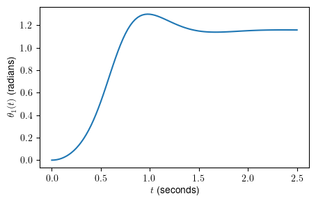
%matplotlib inline

fig, ax = plt.subplots(figsize=(5,3))

ax.plot(sol.t, sol.y[0,:], markeredgewidth=2)
ax.set_xlabel(" $t$ (seconds) ")
ax.set_ylabel(" $\\theta_1 (t) $ (radians) ")
plt.show()

%matplotlib notebook

import matplotlib.pyplot as plt
import numpy as np

import matplotlib.animation as animation

# Collect the points 
N = len(sol.t)
th1_array = sol.y[0,:]
th2_array = RPM_ * sol.t

# Plotting starts here
fig = plt.figure()
ax = fig.add_subplot(projection="3d")

# Create lines initially
E = np.array([0., 0., 0.])  
F = np.array([0., 0., -2*l_])
rod  = ax.plot([E[0], F[0]], [E[1], F[1]], [E[2], F[2]], '-r', linewidth=3.0 )[0]
arms = ax.plot([], [], [], '.-b')[0] # without data

# Setting the Axes properties
ax.set(xlim3d=(-0.2, 0.2), xlabel='X')
ax.set(ylim3d=(-0.2, 0.2), ylabel='Y')
ax.set(zlim3d=(-0.2, 0.2), zlabel='Z')

# --- Animation update callback function ---
def update_lines(num):
    A1 = np.array([-d_*cos(th2_array[num]),-d_*sin(th2_array[num]),0], dtype=np.float32)
    A2 = np.array([ d_*cos(th2_array[num]), d_*sin(th2_array[num]),0], dtype=np.float32)
    B  = np.array([-(l_*sin(th1_array[num])+d_)*cos(th2_array[num]), -(l_*sin(th1_array[num])+d_)*sin(th2_array[num]), -l_*cos(th1_array[num])])
    C  = np.array([(l_*sin(th1_array[num])+d_)*cos(th2_array[num]),  (l_*sin(th1_array[num])+d_)*sin(th2_array[num]), -l_*cos(th1_array[num])])
    D  = np.array([ 0,0, -l_*cos(th1_array[num])*2])
    arms.set_data_3d(np.vstack([D, B, A1, A2, C, D]).T)

    return [arms]
# ---

ani = animation.FuncAnimation(fig, update_lines, N,  interval=1000);
ani.save("./images/flyball.gif",  writer='imagemagick', fps=15);
display_gif("./images/flyball.gif")