The Root-Locus Method#
Given the following closed-loop controlled system:
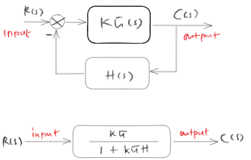
The root locus method draws the location of the closed-loop poles for all \(K \geq 0\).
However, the root-locus method does this by only considering the open-loop transfer function ( \(G(s)H(s)\) ).
Preparations#
Show code cell source
import numpy as np

from sympy import simplify, fraction, solve, expand, Symbol, re, im, Matrix, Eq, diff, latex
from sympy.physics.control.lti import TransferFunction
from sympy.abc import s

from rlocusanim import *

from mathprint import *
The core function for root-locus plotting#
Steps performed:
Define a symbolic positive real gain K.
Build the open-loop transfer function
OL = simplify(G*H)and create a SymPy TransferFunction to extract open-loop poles and zeros.Form the closed-loop transfer function
T(s) = K*G / (1 + K*G*H)and extract its denominator (the characteristic equation).Generate a set of gains (log-spaced from 0.001 up to
Kmax) to sample the locus.For each sampled gain, substitute
Kinto the closed-loop TF and compute the closed-loop poles.Collect the pole locations for each gain to produce the root-locus branches.
Return:
gains,cl_poles(array of pole locations vs gain), ol_poles, ol_zeros.
Practical notes:
Log-spacing concentrates samples at small gains where many changes occur; adjust
numandKmaxto resolve features.Symbolic substitution can be slow for high-order systems.
The returned
cl_polesarray is suitable foranimate(...)to draw pole trajectories.
def rlocus(G, H, Kmax=10000, num=100):
    K = Symbol('K', positive=True, real=True)

    ol_tf = fraction(simplify(G * H));
    ol_TF = TransferFunction(ol_tf[0], ol_tf[1], s)

    ol_poles = np.complex64(ol_TF.poles())
    ol_zeros = np.complex64(ol_TF.zeros())

    cl_tf = fraction(simplify(K*G / (1+K*G*H)))
    cl_TF = TransferFunction(cl_tf[0], cl_tf[1], s)

    cl_poles = []
    gains = np.logspace(np.log10(0.001), np.log10(Kmax), num)
    gains = np.hstack((0, gains))
    for gain in gains:
        p = cl_TF.subs(K, gain).poles()
        cl_poles.append([p[i].evalf() for i in range(len(p))])

    cl_poles = np.complex64(cl_poles)

    return gains, cl_poles, ol_poles, ol_zeros
Finding the \(j\omega\) crossings#
The crossings include the gain \(K\) and frequency \(\omega\) where closed-loop poles lie on the imaginary axis.
For the closed-loop transfer function
the closed-loop poles come from the denominator, also called the characteristic equation:
find_jw_crossings(...) follows these steps:
Define
Kas a positive real symbolic gain andomegaas a real symbolic frequency.Build the closed-loop transfer function
K*G/(1 + K*G*H).Use
fraction(...)to extract the denominator of the simplified closed-loop transfer function. This denominator is the characteristic equation.Substitute
s = j*omegainto that denominator.Split the result into its real and imaginary parts.
Solve these two equations to obtian
Kandomega:\[\operatorname{Re}(D(j\omega)) = 0\]\[\operatorname{Im}(D(j\omega)) = 0\]Display the solutions as a matrix.
If the output contains both positive and negative values of \(\omega\), they represent the conjugate imaginary-axis poles at \(+j\omega\) and \(-j\omega\). Usually the positive frequency is the one reported physically.
def find_jw_crossings(G, H):
    K = Symbol('K', positive=True, real=True)
    omega = Symbol('omega', real=True)

    cl_tf = fraction(simplify(K*G/(1+K*G*H)))
    eq = cl_tf[1].subs(s, omega*1j)

    # Build system equations made by real and immaginary compinents
    eqs = Matrix([re(eq), im(eq)])
    sol = solve(Eq(eqs,Matrix([[0],[0]])), [K,omega])
    sol.insert(0, (K, omega))
    mprint(latex(Matrix(sol)))
Finding break-away / entry points#
Calculated from the characteristic function of the closed-loop-pole transfer function: \(\displaystyle 1 + KG(s) H(s) = 0\).
Express the closed-loop-pole transfer function as: \(K(s)=\dots\) (this should be a polynomial function of \(s\)-variable).
At break away / entry point,\(\displaystyle \frac{ \mathtt{d} K(s)}{ \mathtt{d} s} = 0\). Solve for \(s\). Assume the solutions are \(s=\mathcal{S}\).
To define if the point is valid: \(K(\mathcal{S}) > 0\).
To define whether the point is an entry point or a break-away point:
Entry point: \(\displaystyle \frac{ \mathtt{d}^2K(\mathcal{S})} { \mathtt{d} s^2} > 0\).
Break-away point: \(\displaystyle \frac{ \mathtt{d}^2K(\mathcal{S})}{ \mathtt{d} s^2} < 0\).
def find_break_entry_points(G, H):
    K = Symbol('K', positive=True, real=True)

    cl_tf = fraction(simplify(K*G/(1+K*G*H)))
    eq = solve(cl_tf[1], K)[0]
    deq = diff(eq, s)
    ddeq = diff(eq, s, s)

    sol = solve(deq, s)
    sols = ([re(sol[i].evalf()) for i in range(len(sol))]) # this results should be only real numbers

    S = []
    for s_ in sols:
        K_ = eq.subs(s, s_)
        if K_ > 0:
            S.append(s_)

    STATUS = []
    for s_ in S:
        eq_ = ddeq.subs(s, s_)
        if eq_.evalf() < 0:
            STATUS.append("Break-away point")
        else:
            STATUS.append("Entry point")

    return S, STATUS
Example 1#
Rot-locus plot#
%matplotlib notebook
gains, cl_poles, ol_poles, ol_zeros = rlocus(1/(s**3+s**2+45*s), 1, Kmax=2000);
ani = animate(gains, cl_poles, ol_poles, ol_zeros, gif_fn='./images/1.gif');
display_gif("./images/1.gif");

\(j \omega\)-crossings#
find_jw_crossings(1/(s**3+s**2+45*s), 1)
Example 2#
Root-locus plot#
%matplotlib notebook
gains, cl_poles , ol_poles, ol_zeros = rlocus((s-1)/(s+3), 1)
ani = animate(gains, cl_poles, ol_poles, ol_zeros, gif_fn='./images/2.gif');
display_gif("./images/2.gif");

\(j \omega\)-crossings#
find_jw_crossings((s-1)/(s+3), 1)
Example 3#
Root-locus plot#
%matplotlib notebook
gains, cl_poles , ol_poles, ol_zeros = rlocus(1/(s*(1+0.5*s)*(1+0.1*s)), 1, Kmax=200)
ani = animate(gains, cl_poles, ol_poles, ol_zeros, gif_fn='./images/3.gif', fps=60);
display_gif("./images/3.gif");

\(j \omega\)-crossings#
find_jw_crossings(1/(s*(1+0.5*s)*(1+0.1*s)), 1)
For the shake of curiosity, let us do the calculation by hand.
Substitute \(\displaystyle s=j\omega \), and find the \(\displaystyle \omega \).
We can get two equations: \(\displaystyle -0.6\omega ^{2} +K=0\) and \(\displaystyle -0.05\omega ^{3} +\omega =0.\)
From: \(\displaystyle -0.05\omega ^{3} +\omega =0\Longrightarrow \cancel{\omega =0} \lor \omega =-4.472\lor \omega =4.472\).
\(\displaystyle \omega =0\) does not make any sense.
Take \(\displaystyle \omega =\pm 4.472\), substitute \(\displaystyle \omega \pm 4.472\) to \(\displaystyle -0.6\omega ^{2} +K=0\), and we get \(\displaystyle K=12\).
Break-away / entry points#
S, STATUS = find_break_entry_points(1/(s*(1+0.5*s)*(1+0.1*s)), 1)
print(S)
print(STATUS)
[-0.944949536696107]
['Break-away point']
Example 4#
To get a nice root-locus plot, we need to play a bit with the Kmax and num arguments. Otherwise, our root-locus plot will look funny.
Root-locus plot#
%matplotlib notebook
gains, cl_poles , ol_poles, ol_zeros = rlocus((s+2)*(s+3)/(s*(s+1)), 1, Kmax=100, num=1000)
ani = animate(gains, cl_poles, ol_poles, ol_zeros, gif_fn='./images/4.gif', fps=500);
display_gif("./images/4.gif");

Break-away / entry points#
S, STATUS = find_break_entry_points((s+2)*(s+3)/(s*(s+1)), 1)
print(S)
print(STATUS)
[-2.36602540378444, -0.633974596215561]
['Entry point', 'Break-away point']