PID Control of a First Order System

Preparations

Here we import all necessary libraries.

Show code cell source Hide code cell source

from IPython.core.display import HTML
import numpy as np

import matplotlib.pyplot as plt
plt.rcParams.update({
    "text.usetex": True,
    "font.family": "sans",
    "font.size": 10,
})

from sympy import *
from sympy.plotting import plot

from mathprint import *

These are some variables that we are going to use:

\(t, s, \tau, \omega, \omega_n, \zeta\)

from sympy.physics.control.lti import TransferFunction
Kp, Ki, Kd = symbols('K_p K_i K_d', positive=True)

t       = symbols('t', positive=True)
s       = symbols('s', complex=True)
tau     = symbols('tau', positive=True)

omega   = symbols("omega", positive=True)
omega_n = symbols('omega_n', positive=True)
zeta    = symbols('zeta', positive=True)

Let us define some helper functions.

def laplace(f):
    F = laplace_transform(f, t, s, noconds=True)
    return F

def ilaplace(F):
    f = inverse_laplace_transform(F, s, t)
    return f

def frac_to_tf(frac):
    return TransferFunction(fraction(frac)[0], fraction(frac)[1], s)

System and the control equations

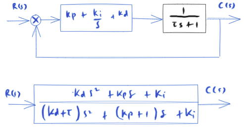
The diagram above corresponds to a unity-feedback loop with

\[ G(s)=K_p+\frac{K_i}{s}+K_d \]

and plant

\[ H(s)=\frac{1}{\tau s+1}. \]

Thus, the closed-loop transfer function is

\[ \frac{C(s)}{R(s)} = \frac{\left(K_p+\frac{K_i}{s}+K_ds\right)\frac{1}{\tau s+1}} {1+\left(K_p+\frac{K_i}{s}+K_ds\right)\frac{1}{\tau s+1}} = \frac{K_d s^2+K_p s+K_i} {(\tau+K_d)s^2+(1+K_p)s+K_i} \]

H = 1 / (tau*s+1)
G = Kp + Ki/s + Kd*s   # PID-control
Q = factor(((G*H / (1 + G*H))))

print("first-order system:")
mprint("H(s)=", latex(H))

print("PID-control:")
mprint("G(s)= ", latex(G))

print("the resulting closed-loop system:")
mprint("Q(s)=", latex(Q))

first-order system:

\[\displaystyle H(s)=\frac{1}{s \tau + 1}\]

PID-control:

\[\displaystyle G(s)= K_{d} s + \frac{K_{i}}{s} + K_{p}\]

the resulting closed-loop system:

\[\displaystyle Q(s)=\frac{K_{d} s^{2} + K_{i} + K_{p} s}{K_{d} s^{2} + K_{i} + K_{p} s + s^{2} \tau + s}\]

First order system with P-control

Closed-loop transfer function:

Qp = simplify(Q.subs(([Kd, 0],
                      [Ki, 0])))

mprint(latex(Qp))

\[\displaystyle \frac{K_{p}}{K_{p} + s \tau + 1}\]

The controlled system remains a first order system. \(K_p\) changes the pole location. New pole location:

Closed-loop poles and zeros

f = frac_to_tf(Qp)
zerosp = f.zeros()
polesp = f.poles()

print("closed-loop zeros:")
mprint(latex(zerosp))
       
print("closed-loop poles:")
mprint(latex(polesp))

closed-loop zeros:

\[\displaystyle \left[ \right]\]

closed-loop poles:

\[\displaystyle \left[ - \frac{K_{p} + 1}{\tau}\right]\]

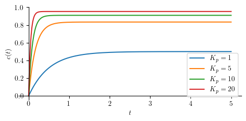
Step response

Let us define some numerical values for our simulations.

tau_ = 1
Kp_  = [1, 5, 10, 20]

We simply perform an inverse Laplace operation to \(C(s)\) and obtain \(c(t)\) as the result. Additionally, we will also compute the steady state-value for the output (\(c_{ss}\)).

cp = ilaplace(Qp * 1/s)

cssp = simplify(limit(cp, t, 'oo'))
c0p  = limit(cp, t, 0)

mprintb("c(t) = ", latex(cp))
mprintb("c_{ss} = ", latex(cssp))

\[\displaystyle \boxed{c(t) = K_{p} \left(- \frac{\tau e^{- \frac{t \left(K_{p}^{2} + 2 K_{p} + 1\right)}{K_{p} \tau + \tau}}}{K_{p} \tau + \tau} + \frac{1}{K_{p} + 1}\right)}\]

\[\displaystyle \boxed{c_{ss} = \frac{K_{p}}{K_{p} + 1}}\]

Show code cell source Hide code cell source

p = [plot(cp.subs(([tau, tau_], [Kp, Kp_[j]])), (t, 0, 5), size=(5, 2.5), ylabel='$c(t)$', show=False, legend=True) for j in range(len(Kp_))]

for j in range(len(p)):
    p[j][0].label = "$K_p=" + str(Kp_[j]) + "$"
    if j > 0:
        p[0].append(p[j][0])

p[0].show()

First-order system with PD-control

Closed-loop transfer function:

Qpd = simplify(Q.subs(Ki, 0))

mprint(latex(Qpd))

\[\displaystyle \frac{K_{d} s + K_{p}}{K_{d} s + K_{p} + s \tau + 1}\]

Closed-loop poles and zeros

f = frac_to_tf(Qpd)
zerospd = f.zeros()
polespd = f.poles()

print("closed-loop zeros:")
mprint(latex(zerospd))

print("closed-loop zeros:")
mprint(latex(polespd))

closed-loop zeros:

\[\displaystyle \left[ - \frac{K_{p}}{K_{d}}\right]\]

closed-loop zeros:

\[\displaystyle \left[ - \frac{K_{p} + 1}{K_{d} + \tau}\right]\]

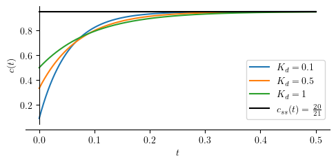
Step response

We simply perform an inverse Laplace operation to \(C(s)\) and obtain \(c(t)\) as the result. Additionally, we will also compute the steady state-value for the output (\(c_{ss}\)).

A phenomenon that can be observed in a derivative control is the “kick” that happens when a step input is applied to the controlled system. Because of the kick, system output does not start from zero.

cpd   = logcombine(ilaplace(Qpd * 1/s))
csspd = limit(cpd, t, 'oo')
c0pd  = limit(cpd, t, 0)

mprintb("c(t) = ", latex(cpd))
mprintb("c_{ss} = ", latex(csspd))
mprintb("c(0) = ", latex(c0pd))

\[\displaystyle \boxed{c(t) = \frac{K_{p}}{K_{p} + 1} + \frac{\left(K_{d} - K_{p} \tau\right) e^{- \frac{t \left(K_{p}^{2} + 2 K_{p} + 1\right)}{K_{d} K_{p} + K_{d} + K_{p} \tau + \tau}}}{K_{d} K_{p} + K_{d} + K_{p} \tau + \tau}}\]

\[\displaystyle \boxed{c_{ss} = \frac{K_{p}}{K_{p} + 1}}\]

\[\displaystyle \boxed{c(0) = \frac{K_{d}}{K_{d} + \tau}}\]

Next, we set up arbitrary numerical values to some parameters and run sumulate the controlled system.

tau_ = 1
Kp_  = 20
Kd_  = [0.1, 0.5, 1]

Show code cell source Hide code cell source

p = [plot(cpd.subs(([tau, tau_], [Kp, Kp_],[Kd, Kd_[j]])), (t, 0, .5), size=(5, 2.5), ylabel='$c(t)$', show=False, legend=True, axis_center=[0,0]) for j in range(len(Kd_))]

for j in range(len(p)):
    p[j][0].label = "$K_d=" + str(Kd_[j]) + "$"
    if j > 0:
        p[0].append(p[j][0])

q = plot(csspd.subs(Kp, Kp_), (t, 0, .5), line_color='k', show=False)

q[0].label = "$ c_{ss} (t) = " + latex(csspd.subs(Kp, Kp_)) + " $"
p[0].append(q[0])
p[0].show()

First-order system with PI-control

Closed-loop transfer function:

Qpi = simplify(Q.subs(Kd, 0))

mprintb(latex(Qpi))

\[\displaystyle \boxed{\frac{K_{i} + K_{p} s}{K_{i} + K_{p} s + s^{2} \tau + s}}\]

Closed-loop poles and zeros

f = frac_to_tf(Qpi)
zerospi = f.zeros()
polespi = f.poles()

print("closed-loop zeros:")
mprint(latex(zerospi))

print("closed-loop zeros:")
mprint(latex(polespi))

closed-loop zeros:

\[\displaystyle \left[ - \frac{K_{i}}{K_{p}}\right]\]

closed-loop zeros:

\[\displaystyle \left[ - \frac{K_{p} + 1}{2 \tau} - \frac{\sqrt{- 4 K_{i} \tau + K_{p}^{2} + 2 K_{p} + 1}}{2 \tau}, \ - \frac{K_{p} + 1}{2 \tau} + \frac{\sqrt{- 4 K_{i} \tau + K_{p}^{2} + 2 K_{p} + 1}}{2 \tau}\right]\]

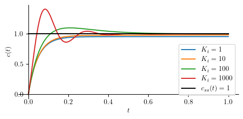
Step response

We simply perform an inverse Laplace operation to \(C(s)\) and obtain \(c(t)\) as the result. Additionally, we will also compute the steady state-value for the output (\(c_{ss}\)).

cpi = ilaplace(Qpi * 1/s)
cpi = sum([simplify(cpi.args[j]) for j in range(len(cpi.args))])

csspi = limit(cpi, t, 'oo')

mprintb("c(t) = ", latex(cpi))
mprintb("c_{ss} = ", latex(csspi))

\[\displaystyle \boxed{c(t) = \frac{\left(K_{p} - 1\right) e^{- \frac{t \left(K_{p} + 1\right)}{2 \tau}} \sin{\left(\frac{t \sqrt{4 K_{i} \tau - K_{p}^{2} - 2 K_{p} - 1}}{2 \tau} \right)}}{\sqrt{4 K_{i} \tau - K_{p}^{2} - 2 K_{p} - 1}} + 1 - e^{- \frac{t \left(K_{p} + 1\right)}{2 \tau}} \cos{\left(\frac{t \sqrt{4 K_{i} \tau - K_{p}^{2} - 2 K_{p} - 1}}{2 \tau} \right)}}\]

\[\displaystyle \boxed{c_{ss} = 1}\]

Next, we set up arbitrary numerical values to some parameters and run sumulate the controlled system.

tau_ = 1
Kp_ = 20
Ki_ = [1, 10, 100, 1000]
Kd_ = 0

Show code cell source Hide code cell source

p = [plot(cpi.subs(([tau, tau_], [Kp, Kp_],[Ki, Ki_[j]])), (t, 0, 1), size=(5, 2.5), ylabel='$c(t)$', show=False, legend=True) for j in range(len(Ki_))]

for j in range(len(p)):
    p[j][0].label = "$K_i=" + str(Ki_[j]) + "$"
    if j > 0:
        p[0].append(p[j][0])

q = plot(csspi.subs(Kp, Kp_), (t, 0, 1), line_color='k', show=False)
q[0].label = "$ c_{ss} (t) = " + latex(csspi.subs(Kp, Kp_)) + " $"
p[0].append(q[0])
p[0].show()

First-order system with PID-control

Closed-loop poles and zeros

f = frac_to_tf(Q)
zerospid = f.zeros()
polespid = f.poles()

print("Closed-loop zeros:")
mprint(latex(zerospid))
       
print("Closed-loop poles:")
mprint(latex(polespid))

Closed-loop zeros:

\[\displaystyle \left[ - \frac{K_{p}}{2 K_{d}} - \frac{\sqrt{- 4 K_{d} K_{i} + K_{p}^{2}}}{2 K_{d}}, \ - \frac{K_{p}}{2 K_{d}} + \frac{\sqrt{- 4 K_{d} K_{i} + K_{p}^{2}}}{2 K_{d}}\right]\]

Closed-loop poles:

\[\displaystyle \left[ - \frac{K_{p} + 1}{2 \left(K_{d} + \tau\right)} - \frac{\sqrt{- 4 K_{d} K_{i} - 4 K_{i} \tau + K_{p}^{2} + 2 K_{p} + 1}}{2 \left(K_{d} + \tau\right)}, \ - \frac{K_{p} + 1}{2 \left(K_{d} + \tau\right)} + \frac{\sqrt{- 4 K_{d} K_{i} - 4 K_{i} \tau + K_{p}^{2} + 2 K_{p} + 1}}{2 \left(K_{d} + \tau\right)}\right]\]

Step response

cpid   = logcombine(ilaplace(Q * 1/s))
csspid = limit(cpid, t, 'oo')
c0pid  = limit(cpid, t, 0)

mprintb("c(t) = ", latex(cpid))
mprintb("c_{ss} = ", latex(csspid))
mprintb("c(0) = ", latex(c0pid))

\[\displaystyle \boxed{c(t) = - \frac{\tau e^{- \frac{t \left(K_{p} + 1\right)}{2 \left(K_{d} + \tau\right)}} \cos{\left(\frac{t \sqrt{K_{d} K_{i} + K_{i} \tau - \frac{K_{p}^{2}}{4} - \frac{K_{p}}{2} - \frac{1}{4}}}{K_{d} + \tau} \right)}}{K_{d} + \tau} + \frac{2 \left(K_{d} + \tau\right) \left(\frac{\tau \left(K_{p} + 1\right)}{2 \left(K_{d} + \tau\right)^{2}} - \frac{1}{K_{d} + \tau}\right) e^{- \frac{t \left(K_{p} + 1\right)}{2 \left(K_{d} + \tau\right)}} \sin{\left(\frac{t \sqrt{4 K_{d} K_{i} + 4 K_{i} \tau - K_{p}^{2} - 2 K_{p} - 1}}{2 \left(K_{d} + \tau\right)} \right)}}{\sqrt{4 K_{d} K_{i} + 4 K_{i} \tau - K_{p}^{2} - 2 K_{p} - 1}} + 1}\]

\[\displaystyle \boxed{c_{ss} = 1}\]

\[\displaystyle \boxed{c(0) = \frac{K_{d}}{K_{d} + \tau}}\]

Compact Engineering Form

Unfortunately, there is no consistently clean automatic SymPy path from a messy ilaplace() result to the compact engineering form

\[ c(t)=c_{DC}+e^{-\sigma t} \left( A\cos(\omega_d t)+B\sin(\omega_d t) \right). \]

Therefore, instead of forcing SymPy to rearrange the expression automatically, we will start from the complete solution for PID control of a first-order system and decompose it manually into three parts:

\[ c(t)=c_1(t)+c_2(t)c_3(t), \]

where \(c_1(t)\) is the DC component, \(c_2(t)\) is the sinusoidal component, and \(c_3(t)\) is the exponential decay envelope.

A0 = Kd + tau
B0 = Kp + 1
C0 = Ki

D = 4*A0*C0 - B0**2

sigma = B0/(2*A0)
omega_d = sqrt(D)/(2*A0)

A = -tau/A0
B = (tau*B0 - 2*A0)/(A0*sqrt(D))

cpid_compact = 1 + exp(-sigma*t)*(A*cos(omega_d*t) + B*sin(omega_d*t))

mprint(r"\sigma = ", latex(sigma))
mprint(r"\omega_d = ", latex(omega_d))
mprint(r"A = ", latex(A))
mprint(r"B = ", latex(B))
mprintb("c(t) = ", latex(cpid_compact))

check = simplify(cpid - cpid_compact)
print("check = ", check)

\[\displaystyle \sigma = \frac{K_{p} + 1}{2 K_{d} + 2 \tau}\]

\[\displaystyle \omega_d = \frac{\sqrt{K_{i} \left(4 K_{d} + 4 \tau\right) - \left(K_{p} + 1\right)^{2}}}{2 K_{d} + 2 \tau}\]

\[\displaystyle A = - \frac{\tau}{K_{d} + \tau}\]

\[\displaystyle B = \frac{- 2 K_{d} + \tau \left(K_{p} + 1\right) - 2 \tau}{\left(K_{d} + \tau\right) \sqrt{K_{i} \left(4 K_{d} + 4 \tau\right) - \left(K_{p} + 1\right)^{2}}}\]

\[\displaystyle \boxed{c(t) = \left(- \frac{\tau \cos{\left(\frac{t \sqrt{K_{i} \left(4 K_{d} + 4 \tau\right) - \left(K_{p} + 1\right)^{2}}}{2 K_{d} + 2 \tau} \right)}}{K_{d} + \tau} + \frac{\left(- 2 K_{d} + \tau \left(K_{p} + 1\right) - 2 \tau\right) \sin{\left(\frac{t \sqrt{K_{i} \left(4 K_{d} + 4 \tau\right) - \left(K_{p} + 1\right)^{2}}}{2 K_{d} + 2 \tau} \right)}}{\left(K_{d} + \tau\right) \sqrt{K_{i} \left(4 K_{d} + 4 \tau\right) - \left(K_{p} + 1\right)^{2}}}\right) e^{- \frac{t \left(K_{p} + 1\right)}{2 K_{d} + 2 \tau}} + 1}\]

check =  0

c_lst = Add.make_args(cpid_compact) # separate cn
c1 = c_lst[0]
c2 = numer(c_lst[1])
c3 = 1 / denom(c_lst[1])

mprintb('c_{1}(t)=', latex(c1))
mprintb('c_{2}(t)=', latex(c2))
mprintb('c_{3}(t)=', latex(c3))

\[\displaystyle \boxed{c_{1}(t)=1}\]

\[\displaystyle \boxed{c_{2}(t)=- \frac{\tau \cos{\left(\frac{t \sqrt{K_{i} \left(4 K_{d} + 4 \tau\right) - \left(K_{p} + 1\right)^{2}}}{2 K_{d} + 2 \tau} \right)}}{K_{d} + \tau} + \frac{\left(- 2 K_{d} + \tau \left(K_{p} + 1\right) - 2 \tau\right) \sin{\left(\frac{t \sqrt{K_{i} \left(4 K_{d} + 4 \tau\right) - \left(K_{p} + 1\right)^{2}}}{2 K_{d} + 2 \tau} \right)}}{\left(K_{d} + \tau\right) \sqrt{K_{i} \left(4 K_{d} + 4 \tau\right) - \left(K_{p} + 1\right)^{2}}}}\]

\[\displaystyle \boxed{c_{3}(t)=e^{- \frac{t \left(K_{p} + 1\right)}{2 K_{d} + 2 \tau}}}\]

Summary

Show code cell source Hide code cell source

from pandas import DataFrame, set_option
from IPython.display import Markdown, display

def makelatex(args):
    return ["${}$".format(latex(a)) for a in args]

descs = ["P", 
         "PD",
         "PI",
         "PID"]

css_label = [cssp, csspd, csspi, csspid]
c_label   = [cp, cpd, cpi, cpid]
cl_zeros  = [zerosp, zerospd, zerospi, zerospid]
cl_poles  = [polesp, polespd, polespi, polespid]
kicks     = [0, c0pd, 0, c0pid]


dic1 = {''         : makelatex(descs), 
        '$c_{ss}$' : makelatex(css_label),
        '$c(0)$'   : makelatex(kicks)}

dic2 = {''         : makelatex(descs), 
        'Zeros'    : makelatex(cl_zeros),
        'Poles'    : makelatex(cl_poles)}

df1 = DataFrame(dic1)
df2 = DataFrame(dic2)

Initial and steady-state output for unit-step input

Show code cell source Hide code cell source

Markdown(df1.to_markdown(index=False))

	\(c_{ss}\)	\(c(0)\)
\(\mathtt{\text{P}}\)	\(\frac{K_{p}}{K_{p} + 1}\)	\(0\)
\(\mathtt{\text{PD}}\)	\(\frac{K_{p}}{K_{p} + 1}\)	\(\frac{K_{d}}{K_{d} + \tau}\)
\(\mathtt{\text{PI}}\)	\(1\)	\(0\)
\(\mathtt{\text{PID}}\)	\(1\)	\(\frac{K_{d}}{K_{d} + \tau}\)

Zeros and poles

Show code cell source Hide code cell source

Markdown(df2.to_markdown(index=False))

	Zeros	Poles
\(\mathtt{\text{P}}\)	\(\left[ \right]\)	\(\left[ - \frac{K_{p} + 1}{\tau}\right]\)
\(\mathtt{\text{PD}}\)	\(\left[ - \frac{K_{p}}{K_{d}}\right]\)	\(\left[ - \frac{K_{p} + 1}{K_{d} + \tau}\right]\)
\(\mathtt{\text{PI}}\)	\(\left[ - \frac{K_{i}}{K_{p}}\right]\)	\(\left[ - \frac{K_{p} + 1}{2 \tau} - \frac{\sqrt{- 4 K_{i} \tau + K_{p}^{2} + 2 K_{p} + 1}}{2 \tau}, \ - \frac{K_{p} + 1}{2 \tau} + \frac{\sqrt{- 4 K_{i} \tau + K_{p}^{2} + 2 K_{p} + 1}}{2 \tau}\right]\)
\(\mathtt{\text{PID}}\)	\(\left[ - \frac{K_{p}}{2 K_{d}} - \frac{\sqrt{- 4 K_{d} K_{i} + K_{p}^{2}}}{2 K_{d}}, \ - \frac{K_{p}}{2 K_{d}} + \frac{\sqrt{- 4 K_{d} K_{i} + K_{p}^{2}}}{2 K_{d}}\right]\)	\(\left[ - \frac{K_{p} + 1}{2 \left(K_{d} + \tau\right)} - \frac{\sqrt{- 4 K_{d} K_{i} - 4 K_{i} \tau + K_{p}^{2} + 2 K_{p} + 1}}{2 \left(K_{d} + \tau\right)}, \ - \frac{K_{p} + 1}{2 \left(K_{d} + \tau\right)} + \frac{\sqrt{- 4 K_{d} K_{i} - 4 K_{i} \tau + K_{p}^{2} + 2 K_{p} + 1}}{2 \left(K_{d} + \tau\right)}\right]\)

Resulting second order system

Show code cell source Hide code cell source

mprintb("c(t) = ", latex(cpid_compact))

print("--- or ---")

mprint('c(t)=c_1(t)+c_2(t)c_3(t)')

mprintb('c_{1}(t)=', latex(c1))
mprintb('c_{2}(t)=', latex(c2))
mprintb('c_{3}(t)=', latex(c3))

\[\displaystyle \boxed{c(t) = \left(- \frac{\tau \cos{\left(\frac{t \sqrt{K_{i} \left(4 K_{d} + 4 \tau\right) - \left(K_{p} + 1\right)^{2}}}{2 K_{d} + 2 \tau} \right)}}{K_{d} + \tau} + \frac{\left(- 2 K_{d} + \tau \left(K_{p} + 1\right) - 2 \tau\right) \sin{\left(\frac{t \sqrt{K_{i} \left(4 K_{d} + 4 \tau\right) - \left(K_{p} + 1\right)^{2}}}{2 K_{d} + 2 \tau} \right)}}{\left(K_{d} + \tau\right) \sqrt{K_{i} \left(4 K_{d} + 4 \tau\right) - \left(K_{p} + 1\right)^{2}}}\right) e^{- \frac{t \left(K_{p} + 1\right)}{2 K_{d} + 2 \tau}} + 1}\]

--- or ---

\[\displaystyle c(t)=c_1(t)+c_2(t)c_3(t)\]

\[\displaystyle \boxed{c_{1}(t)=1}\]

\[\displaystyle \boxed{c_{2}(t)=- \frac{\tau \cos{\left(\frac{t \sqrt{K_{i} \left(4 K_{d} + 4 \tau\right) - \left(K_{p} + 1\right)^{2}}}{2 K_{d} + 2 \tau} \right)}}{K_{d} + \tau} + \frac{\left(- 2 K_{d} + \tau \left(K_{p} + 1\right) - 2 \tau\right) \sin{\left(\frac{t \sqrt{K_{i} \left(4 K_{d} + 4 \tau\right) - \left(K_{p} + 1\right)^{2}}}{2 K_{d} + 2 \tau} \right)}}{\left(K_{d} + \tau\right) \sqrt{K_{i} \left(4 K_{d} + 4 \tau\right) - \left(K_{p} + 1\right)^{2}}}}\]

\[\displaystyle \boxed{c_{3}(t)=e^{- \frac{t \left(K_{p} + 1\right)}{2 K_{d} + 2 \tau}}}\]