Gain Margin and Phase Margin

Preparations

from IPython.core.display import HTML
import numpy as np

import matplotlib.pyplot as plt
plt.rcParams.update({
    "text.usetex": True,
    "font.family": "Helvetica",
    "font.size": 10,
})

from sympy import *
from sympy.plotting import plot
import mpmath as mp

from mathprint import *

Define variables that we are going to use repetitively. We also need to define specific prpoperties of the variables.

from sympy.abc import s, epsilon, k

t        = symbols('t'       , real=True)
omega    = symbols('omega'   , positive=True)
zeta     = symbols('zeta'    , real=True)
omega_n  = symbols('omega_n' , positive=True)

Example 1

Let us take an example that can be found in this MATLAB help page.

Given the system \(G(s)\). We are going to apply a constant gain feedback control to \(G(s)\).

G = (0.5*s + 1.3) / (s**3 + 1.2*s**2 + 1.6*s)
mprint("G(s)=", latex(G))

\[\displaystyle G(s)=\frac{0.5 s + 1.3}{s^{3} + 1.2 s^{2} + 1.6 s}\]

Gjw = G.subs(s, I*omega)
mprint("G(j \\omega)=", latex(Gjw))

\[\displaystyle G(j \omega)=\frac{0.5 i \omega + 1.3}{- i \omega^{3} - 1.2 \omega^{2} + 1.6 i \omega}\]

The magnitude equation:

M = Abs(Gjw)
mprint("M=", latex(M))

Mdb = 20*log(M,10)
mprint("M_{dB} = ", latex(Mdb))

\[\displaystyle M=\frac{0.8125 \sqrt{0.14792899408284 \omega^{2} + 1}}{\sqrt{0.390625 \omega^{6} - 0.6875 \omega^{4} + \omega^{2}}}\]

\[\displaystyle M_{dB} = \frac{20 \log{\left(\frac{0.8125 \sqrt{0.14792899408284 \omega^{2} + 1}}{\sqrt{0.390625 \omega^{6} - 0.6875 \omega^{4} + \omega^{2}}} \right)}}{\log{\left(10 \right)}}\]

The phase equation:

Phi = simplify(atan(im(Gjw)/re(Gjw)))
mprint("\\phi = ", latex(Phi))

\[\displaystyle \phi = \operatorname{atan}{\left(\frac{2.08 - 0.7 \omega^{2}}{\omega \left(0.5 \omega^{2} + 0.76\right)} \right)}\]

Cross-over frequencies

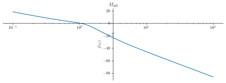
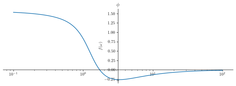
Bode plot

mag = plot(Mdb, (omega, 0.1 , 100), size=(8, 3), show=False, title='$ M_{dB} $', xscale='log')
mag.show()

pha = plot(Phi, (omega, 0.1 , 100), size=(8, 3), title='$ \\phi $', show=False,  xscale='log')
pha.show()

Gain cross-over frequency

Find \(\omega\) where the magnitude is zero dB. Take the positive value.

w_gain = list(solveset(Eq(Mdb, 0), omega, domain=S.Reals))
mprint("\\omega_{gain}=", latex(w_gain))

\[\displaystyle \omega_{gain}=\left[ -1.03642323216522, \ 1.03642323216522\right]\]

Phase cross-over frequency

Find \(\omega\) where the phase is \(n\pi\), where \(n\) is integer numbers (negative, zero, and positive). From the plot, we know we must check 0. Take the positive value.

w_phase = list(solveset(Eq(Phi, 0), omega, domain=S.Reals))
mprint("\\omega_{phase}=", latex(w_phase))

\[\displaystyle \omega_{phase}=\left[ -1.72378321474267, \ 1.72378321474267\right]\]

Gain margin

\(M_{dB}\) when \(\omega = \omega_{phase}\)

GM = abs(Mdb.subs(omega, w_phase[1]).evalf())
GM

\[\displaystyle 8.76406377378585\]

Phase margin

\(\phi\) when \(\omega = \omega_{gain}\)

PM = abs(mp.degrees(Phi.subs(omega, w_gain[1]).evalf())) # in  degrees
PM

\[\displaystyle 44.651569314662\]

Comparison with the Routh method

Let us take a look at the gain margin. Since it is in dB, let us bring it back to a plain gain.

mprintb(latex(10**(GM/20)))

\[\displaystyle \boxed{2.74285714285714}\]

Now, let us apply the Routh method for the closed-loop system. Hence, first we must compute the closed-loop transfer function.

Gcl = simplify(k*G/(1+k*G))
Gcl

\[\displaystyle \frac{k \left(0.5 s + 1.3\right)}{k \left(0.5 s + 1.3\right) + s^{3} + 1.2 s^{2} + 1.6 s}\]

Now, we can apply the Routh method.

from rh import *

table = make_routh_table(Gcl)
print_table(table)

\[\begin{split}\displaystyle \left[\begin{matrix}1.0 & 0.5 k + 1.6 & 0\\1.2 & 1.3 k & 0\\1.6 - 0.583333333333333 k & 0 & 0\\1.3 k & 0 & 0\end{matrix}\right]\end{split}\]

Our concern is at row #3 and column #1. This part can not be zero or negative. Knowing this, we can then compute the maximum value for \(k\).

table[2,0]

\[\displaystyle 1.6 - 0.583333333333333 k\]

reduce_inequalities(table[2,0] > 0, k)

\[\displaystyle -\infty < k \wedge k < 2.74285714285714\]

\[ \boxed{\text{The value is exacly identical with the gain margin that we have previously computed!}} \]