Linear Support Vector Machine

This material is heavily based on the popular Standford CS231n lecture material. Please check on their website for more detailed information.

import numpy as np
import matplotlib.pyplot as plt

plt.rcParams.update({
    "text.usetex": True,
    "font.family": "sans-serif",
    "font.size": 10,
})

from utils import *

np.set_printoptions(precision=5, suppress=True)

Class SVM

This is the Python class implementation of the linear SVM:

• There two metods: train(X, Y) and Y = predict(X).

• Matrix self.W also includes the bias vector (bias tricks).

• Training is done by using stochastic gradient descent method or gradient descent method.

Let us define the score function as linear combination of all feature values.

\( F = X W \)

\(L_i = \sum_{j \neq Y_i} \max(0, F_{i,j}-F_{i,Y_i} + 1)\)

\( L=\underbrace{\frac{1}{N} \sum_{i=1}^N L_{i}}_{\text {data loss }}+\underbrace{\lambda R(W)}_{\text {regularization loss }} \)

\( R(W) = \sum_{k=1}^C \sum_{l=1}^{D+1} W_{l, k}^{2} \)

where:

• the dataset contains \(N\) samples of data

• each sample has \(D\) features (dimensionalities) and \(C\) labels/classes (distinct categories)

• \(X \in \mathbb{R}^{N \times (D+1)}\) contains the features from N samples of data

• \(X_i \in \mathbb{R}^{D+1}\) contains the features of the \(i\)-th sample (\(i\)-th row of \(X\))

• \(Y \in \mathbb{R}^{N}\) contains the correct classes from N samples of data

• \(Y_i \in \mathbb{R}\) contains the correct class of the \(i\)-th sample (\(i\)-th row of \(Y\))

• \(F_{i,j} \in \mathbb{R}\) is the score for \(i\)-th sample and \(j\)-th class (\(i\)-th row and \(j\)-th column)

• \(F_{i,Y_i} \in \mathbb{R}\) is the score for the correct class of \(i\)-th sample

• \(L \in \mathbb{R}\) is the total loss

• \(L_i \in \mathbb{R}\) is the loss of \(i\)-th sample

• \(W \in \mathbb{R}^{(D+1) \times C}\) is the weight matrix (with augmented bias vector in the last row)

• \(R \in \mathbb{R}\) is the regularization loss

Note: the words “label” and “class” have similar meaning!

from numba import njit, prange

class SVM():
    @staticmethod
    @njit(parallel=True, fastmath=True)
    def svm_loss(W, X, Y, reg):
        """
        Structured SVM loss function, naive implementation (with loops).

        Inputs have dimension D, there are C classes, and we operate on minibatches
        of N examples.

        Inputs:
        - W: A numpy array of shape (D+1, C) containing weights.
        - X: A numpy array of shape (N, D) containing a minibatch of data.
        - Y: A numpy array of shape (N,) containing training labels; y[i] = c means
          that X[i] has label c, where 0 <= c < C.
        - reg: (float) regularization strength

        Returns a tuple of:
        - loss: loss as single float
        - dW: gradient with respect to weights W; an array of same shape as W

        References:
        - https://github.com/lightaime/cs231n
        - https://github.com/mantasu/cs231n
        - https://github.com/jariasf/CS231n

        """
        X  = np.hstack((X, np.ones((X.shape[0],1)))) # the last column is 1: to allow augmentation of bias vector into W

        dW = np.zeros(W.shape)  # initialize the gradient as zero

        # compute the loss and the gradient
        C = W.shape[1]
        N = X.shape[0]
        loss = 0.0

        F = X@W
        for i in prange(N):
            Fi = F[i]
            Fyi = Fi[Y[i]]
            Li = Fi - Fyi + 1        # 
            Li[np.where(Li < 0)] = 0 # max(0, ...)
            loss += np.sum(np.delete(Li, Y[i]))

            for j in prange(C):         
                if Li[j] > 0 and j != Y[i]:
                    dW[:, j] += X[i]    # update gradient for incorrect label
                    dW[:, Y[i]] -= X[i] # update gradient for correct label

        loss  = loss / N + reg * np.sum(W * W) # add regularization to the loss.
        dW = dW / N + 2 * reg * W # append partial derivative of regularization term

        return loss, dW


    @staticmethod
    def svm_loss_vectorized(W, X, Y, reg):
        """
        Structured SVM loss function, naive implementation (with loops).

        Inputs have dimension D, there are C classes, and we operate on minibatches
        of N examples.

        Inputs:
        - W: A numpy array of shape (D+1, C) containing weights.
        - X: A numpy array of shape (N, D) containing a minibatch of data.
        - Y: A numpy array of shape (N,) containing training labels; y[i] = c means
          that X[i] has label c, where 0 <= c < C.
        - reg: (float) regularization strength

        Returns a tuple of:
        - loss: loss as single float
        - dW: gradient with respect to weights W; an array of same shape as W

        References:
        - https://github.com/lightaime/cs231n
        - https://github.com/mantasu/cs231n
        - https://github.com/jariasf/CS231n

        """
        X  = np.hstack((X, np.ones((X.shape[0],1)))) # the last column is 1: to allow augmentation of bias vector into W
        N = X.shape[0]

        # scores
        F  = X @ W

        # Scores for correct labels
        Fy = F[range(N), Y].reshape(-1,1)

        # compute the loss
        L  = F - Fy + 1
        L  = np.maximum(0, L) # max(0, ...)
        L_ = L.copy() # keep the original
        L[range(N) , Y] = 0 # exclude the correct labels
        loss = np.sum(L) / N + reg * np.sum(W * W)

        # compute the gradient
        dW = (L_ > 0).astype(float) # positive for incorrect labels
        dW[range(N), Y] = dW[range(N), Y] - dW.sum(axis=1) # negative for correct labels
        dW = X.T @ dW / N + 2 * reg * W  # gradient with respect to W

        return (loss, dW)
      

    def train(self, X, Y, learning_rate=1e-3, reg=1e-5, num_iters=100, batch_size=200, verbose=True, verbose_step=1000):
        '''
        Train this linear classifier using stochastic gradient descent. 
        Setting the 'batch_size=None" turns of the stochastic feature.

        Inputs:
        - X: A numpy array of shape (N, D) containing training data; there are N
          training samples each of dimension D.
        - y: A numpy array of shape (N,) containing training labels; y[i] = c
          means that X[i] has label 0 <= c < C for C classes.
        - learning_rate: (float) learning rate for optimization.
        - reg: (float) regularization strength.
        - num_iters: (integer) number of steps to take when optimizing
        - batch_size: (integer) number of training examples to use at each step.
        - verbose: (boolean) If true, print progress during optimization.
        - verbose_steps: (integer) print proress once every verbose_steps

        Outputs:
        A list containing the value of the loss function at each training iteration.
        '''
          
        N, D = X.shape
        C = len(np.unique(Y)) 
        
        # lazily initialize W
        self.W = 0.001 * np.random.randn(D + 1, C) # dim+1, to bias vector is augmented into W 

        # Run stochastic gradient descent to optimize W
        loss_history = []
        for it in range(num_iters):
            X_batch = None
            y_batch = None

            # Sample batch_size elements from the training data and their           
            # corresponding labels to use in this round of gradient descent.        
            # Store the data in X_batch and their corresponding labels in           
            # y_batch; after sampling X_batch should have shape (dim, batch_size)   
            # and y_batch should have shape (batch_size,)                           
            
            if batch_size is not None:
                batch_indices = np.random.choice(N, batch_size, replace=False)
                X_batch = X[batch_indices]
                y_batch = Y[batch_indices]
                loss, grad = self.svm_loss_vectorized(self.W, X_batch, y_batch, reg)
            else:
                loss, grad = self.svm_loss_vectorized(self.W, X, Y, reg)
            
            loss_history.append(loss)

            # Update the weights using the gradient and the learning rate.          
            self.W = self.W - learning_rate * grad
     
            if verbose and it % verbose_step == 0 or it == num_iters - 1:
                print('iteration %d / %d: loss %f' % (it, num_iters, loss), flush=True)

        return loss_history
    

    def predict(self, X):
        """
        Use the trained weights of this linear classifier to predict labels for
        data points.

        Inputs:
        - X: A numpy array of shape (N, D) containing training data; there are N
          training samples each of dimension D.

        Returns:
        - Y_pred: Predicted labels for the data in X. y_pred is a 1-dimensional
          array of length N, and each element is an integer giving the predicted
          class.
        """
        
        X  = np.hstack((X, np.ones((X.shape[0],1))))

        Y_pred = np.zeros(X.shape[0])
        scores = X @ self.W
        Y_pred = scores.argmax(axis=1)

        return Y_pred

Breast Cancer Wisconsin

This dataset is publicly available and can be downloaded from this link.

This dataset is also available as one of scikit-learn example datasets.

The original labels are characters: M and B. For the SVM to work, the labels must be numbers. Hence, we change the labels:

• M is replaced with 1

• B is replaced with 0

Load the Dataset

data = np.loadtxt("./datasets/breast_cancer/wdbc.data", delimiter=",", dtype=str)
X = np.float32(data[:, 2:12])  # 10 dimensions

# Diagnosis (M = malignant, B = benign)
Y = np.zeros(X.shape[0], dtype=np.int32) 
Y[np.where(data[:,1]=='M')] = 1
Y[np.where(data[:,1]=='B')] = 0

print("Dimension numbers :", X.shape[1])
print("Number of data    :", X.shape[0])
print("Labels            :", np.unique(Y))

Dimension numbers : 10
Number of data    : 569
Labels            : [0 1]

Split The Dataset for Training and Test

X_train = X[0:400, :]
y_train = Y[0:400]
X_test  = X[401:, :]
Y_test  = Y[401:]

num_test = X_test.shape[0]

Train the Classifier

classifier = SVM()
loss_hist = classifier.train(X_train, y_train, learning_rate=1e-6,batch_size=200, reg=1, num_iters=20000, verbose_step=2000)

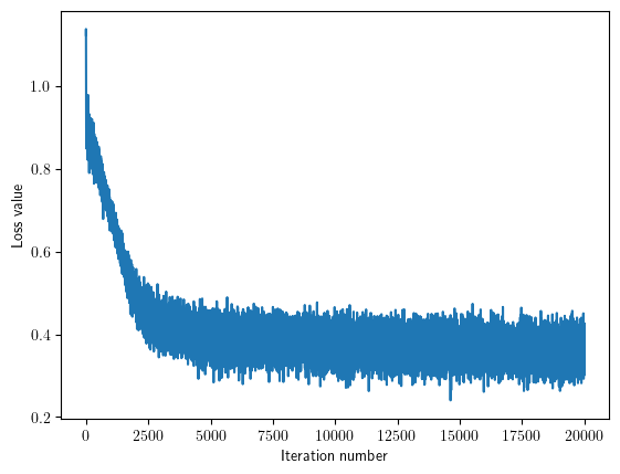
iteration 0 / 20000: loss 1.122593

iteration 2000 / 20000: loss 0.501769

iteration 4000 / 20000: loss 0.433979

iteration 6000 / 20000: loss 0.365286

iteration 8000 / 20000: loss 0.363138

iteration 10000 / 20000: loss 0.392463

iteration 12000 / 20000: loss 0.349064

iteration 14000 / 20000: loss 0.355593

iteration 16000 / 20000: loss 0.414111

iteration 18000 / 20000: loss 0.355115

iteration 19999 / 20000: loss 0.328130

Plot the Loss

Plot the loss as a function of iteration number.

plt.plot(loss_hist)
plt.xlabel('Iteration number')
plt.ylabel('Loss value')
plt.show()

Test the Classifier

Evaluate the performance on both the training and validation set.

Y_train_pred = classifier.predict(X_train)
print('training accuracy: %f' % (np.mean(y_train == Y_train_pred), ))
Y_test_pred = classifier.predict(X_test)
print('validation accuracy: %f' % (np.mean(Y_test == Y_test_pred), ))

training accuracy: 0.857500
validation accuracy: 0.892857

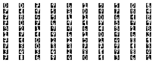
Handwritten Digits

This dataset is publicly available and can be downloaded from this link.

Training Data

data = np.loadtxt("./datasets/handwritten_digits/optdigits.tra", delimiter=",", dtype=int)
X_train = np.int32(data[:, 0:-1])  
y_train = np.int32(data[:, -1]) 

print("Dimension numbers :", X_train.shape[1])
print("Number of data    :", X_train.shape[0])
print("Labels            :", np.unique(y_train))

Dimension numbers : 64
Number of data    : 3823
Labels            : [0 1 2 3 4 5 6 7 8 9]

Test Data

for i in range(100):
    X_train_ = X_train[i,:].reshape(8, 8)
    X_train_ = np.abs(255.0 - 255.0 / 16.0 * X_train_)
    plt.subplot(20, 10, i + 1)
    # Rescale the weights to be between 0 and 255
    plt.imshow(X_train_.astype('uint8'), cmap='Greys')
    plt.axis('off')

data = np.loadtxt("./datasets/handwritten_digits/optdigits.tes", delimiter=",", dtype=int)
X_test = np.int32(data[:, 0:-1])  
y_test = np.int32(data[:, -1]) 

print("Dimension numbers :", X_test.shape[1])
print("Number of data    :", X_test.shape[0])
print("Labels            :", np.unique(y_test))

Dimension numbers : 64
Number of data    : 1797
Labels            : [0 1 2 3 4 5 6 7 8 9]

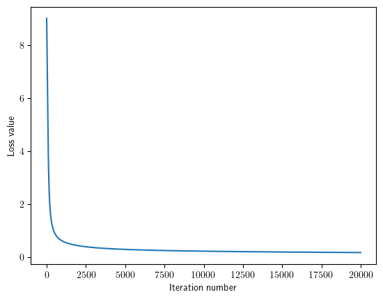
Train the Classifier

classifier = SVM()
loss_hist = classifier.train(X_train, y_train, learning_rate=1e-5, batch_size=None, num_iters=20000, verbose_step=5000)

iteration 0 / 20000: loss 9.024547

iteration 5000 / 20000: loss 0.289658

iteration 10000 / 20000: loss 0.222047

iteration 15000 / 20000: loss 0.191010

iteration 19999 / 20000: loss 0.171675

Plot the Loss

Plot the loss as a function of iteration number.

plt.plot(loss_hist)
plt.xlabel('Iteration number')
plt.ylabel('Loss value')
plt.show()

Test the Classifier

Evaluate the performance on both the training and validation set.

y_train_pred = classifier.predict(X_train)
print('training accuracy: %f' % (np.mean(y_train == y_train_pred), ))
y_test_pred = classifier.predict(X_test)
print('validation accuracy: %f' % (np.mean(y_test == y_test_pred), ))

training accuracy: 0.966780
validation accuracy: 0.933779

Visualize the Learned Weights

• Take matrix W and strip out the bias.

• For each class, reshape the matrix back into 2D arrays

• Plot the 2D arrays (matrices) as images.

w = classifier.W[:-1, :] # strip out the bias
w = w.reshape(8, 8, 10)
w_min, w_max = np.min(w), np.max(w)
classes = ['0', '1', '2', '3', '4', '5', '6', '7', '8', '9']
for i in range(10):
    plt.subplot(2, 5, i + 1)
      
    # Rescale the weights to be between 0 and 255
    wimg = 255.0 * (w[:, :, i].squeeze() - w_min) / (w_max - w_min)
    plt.imshow(wimg.astype('uint8'), cmap='Greys')
    plt.axis('off')
    plt.title(classes[i])