Softmax Classifier

This material is heavily based on the popular Standford CS231n lecture material. Please check on their website for more detailed information.

import numpy as np
import matplotlib.pyplot as plt

plt.rcParams.update({
    "text.usetex": False,
    "font.family": "sans-serif",
    "font.size": 10,
})

from utils import *

np.set_printoptions(precision=5, suppress=True)

Class Softmax

This is the implementation of the linear Softmax classifier:

• The Python class has two metods: train(X, Y) and Y = predict(X).

• Matrix self.W is the weight matrix and also includes the bias vector (bias tricks).

• Training is done by using stochastic gradient descent method or gradient descent method.

Let us define the score function as linear combination of all feature values.

\( F = X W\)

\( \text{softmax}(i) = e^{F_{Y_{i}}} \Big/ \sum_{j=1}^C e^{F_{i}} \)

\( L_{i}=-\log \left( \text{softmax}(i) \right) \)

\( L=\underbrace{\frac{1}{N} \sum_{i=1}^N L_{i}}_{\text {data loss }}+\underbrace{\lambda R(W)}_{\text {regularization loss }} \)

\( R(W) = \sum_{k=1}^C \sum_{l=1}^{D+1} W_{l, k}^{2} \)

where:

• the dataset contains \(N\) samples of data

• each sample has \(D\) features (dimensionalities) and \(C\) labels/classes (distinct categories)

• \(X \in \mathbb{R}^{N \times (D+1)}\) contains the features from N samples of data

• \(X_i \in \mathbb{R}^{D+1}\) contains the features of the \(i\)-th sample (\(i\)-th row of \(X\))

• \(Y \in \mathbb{R}^{N}\) contains the labels from N samples of data

• \(Y_i \in \mathbb{R}\) contains the label of the \(i\)-th sample (\(i\)-th row of \(Y\))

• \(F_i \in \mathbb{R}^{C}\) is the scores for all classes of \(i\)-th sample

• \(F_{y_i} \in \mathbb{R}\) is the score for the correct class of \(i\)-th sample

• \(L \in \mathbb{R}\) is the total loss

• \(L_i \in \mathbb{R}\) is the loss of \(i\)-th sample

• \(W \in \mathbb{R}^{(D+1) \times C}\) is the weight matrix (with augmented bias vector in the last row)

• \(R \in \mathbb{R}\) is the regularization loss

from numba import njit, prange

class Softmax():
    @staticmethod
    @njit(parallel=True, fastmath=True)
    def softmax_loss(W, X, Y, reg):
        """
        Inputs have dimension D, there are C classes, and we operate on minibatches
        of N examples.

        Inputs:
        - W: A numpy array of shape (D+1, C) containing weights.
        - X: A numpy array of shape (N, D) containing a minibatch of data.
        - Y: A numpy array of shape (N,) containing training labels; Y[i] = c means
          that X[i] has label c, where 0 <= c < C.
        - reg: (float) regularization strength

        Returns a tuple of:
        - loss: loss as single float
        - dW: gradient with respect to weights W; an array of same shape as W

        References:
        - https://github.com/lightaime/cs231n
        - https://github.com/mantasu/cs231n
        - https://github.com/jariasf/CS231n
        
        """
        # Initialize the loss and gradient to zero.
        loss = 0.0
        dW   = np.zeros_like(W)
        
        N = X.shape[0] # samples 
        C = W.shape[1] # classes
        X = np.hstack((X, np.ones((N, 1)))) # the last column is 1: to allow augmentation of bias vector into W

        F = X@W 

        # Softmax Loss
        for i in prange(N):
            Fi = F[i] - np.max(F[i])
            expFi = np.exp(Fi)
            softmax = expFi/np.sum(expFi) 
            loss += -np.log(softmax[Y[i]])

            # Weight Gradients
            for j in prange(C):
                dW[:, j] += X[i] * softmax[j]
            dW[:, Y[i]] -= X[i]

        # Average and regulation
        loss = loss /  N + reg * np.sum(W * W)
        dW = dW / N + reg * 2 * W 

        return loss, dW
    
    
    @staticmethod
    def softmax_loss_vectorized(W, X, Y, reg):
        """
        Inputs have dimension D, there are C classes, and we operate on minibatches
        of N examples.

        Inputs:
        - W: A numpy array of shape (D+1, C) containing weights.
        - X: A numpy array of shape (N, D) containing a minibatch of data.
        - Y: A numpy array of shape (N,) containing training labels; Y[i] = c means
          that X[i] has label c, where 0 <= c < C.
        - reg: (float) regularization strength

        Returns a tuple of:
        - loss: loss as single float
        - dW: gradient with respect to weights W; an array of same shape as W

        References:
        - https://github.com/lightaime/cs231n
        - https://github.com/mantasu/cs231n
        - https://github.com/jariasf/CS231n
        
        """
        # Initialize the loss and gradient to zero.
        loss = 0.0
        dW   = np.zeros_like(W)
        
        N = X.shape[0] # samples 
        C = W.shape[1] # classes
        X = np.hstack((X, np.ones((N, 1)))) # the last column is 1: to allow augmentation of bias vector into W

        F = X@W 
        
        # Softmax Loss
        F = F - np.max(F, axis=1).reshape(-1,1)
        expF = np.exp(F)
        softmax = expF/np.sum(expF, axis=1).reshape(-1,1) 
        loss = np.sum(-np.log(softmax[range(N),Y])) / N + reg * np.sum(W * W)

        # derivative of the loss
        softmax[range(N), Y] -= 1                  # update the softmax table
        dW = X.T @ softmax / N + 2 * reg * W       # calculate gradient

        return loss, dW

    
    def train(self, X, Y, learning_rate=1e-3, reg=1, num_iters=100, batch_size=200, verbose=True, verbose_step=1000):
        '''
        Train this linear classifier using stochastic gradient descent.
        Setting the 'batch_size=None" turns of the stochastic feature.

        Inputs:
        - X: A numpy array of shape (N, D) containing training data; there are N
          training samples each of dimension D.
        - Y: A numpy array of shape (N,) containing training labels; y[i] = c
          means that X[i] has label 0 <= c < C for C classes.
        - learning_rate: (float) learning rate for optimization.
        - reg: (float) regularization strength.
        - num_iters: (integer) number of steps to take when optimizing
        - batch_size: (integer) number of training examples to use at each step.
        - verbose: (boolean) If true, print progress during optimization.
        - verbose_steps: (integer) print proress once every verbose_steps

        Outputs:
        A list containing the value of the loss function at each training iteration.
        '''
          
        N, D = X.shape
        C = len(np.unique(Y)) 
        
        # lazily initialize W
        self.W = 0.001 * np.random.randn(D+1, C) # dim+1, to bias vector is augmented into W 

        # Run stochastic gradient descent to optimize W
        loss_history = []
        for it in range(num_iters):
            X_batch = None
            y_batch = None

            # Sample batch_size elements from the training data and their           
            # corresponding labels to use in this round of gradient descent.        
            # Store the data in X_batch and their corresponding labels in           
            # y_batch; after sampling X_batch should have shape (dim, batch_size)   
            # and y_batch should have shape (batch_size,)                           
            
            if batch_size is not None:
              batch_indices = np.random.choice(N, batch_size, replace=False)
              X_batch = X[batch_indices]
              y_batch = Y[batch_indices]
              loss, grad = self.softmax_loss_vectorized(self.W, X_batch, y_batch, reg)
            else:
              loss, grad = self.softmax_loss_vectorized(self.W, X, Y, reg)
            
            loss_history.append(loss)

            # Update the weights using the gradient and the learning rate.          
            self.W = self.W - learning_rate * grad
     
            if verbose and it % verbose_step == 0 or (it == num_iters - 1):
                print('iteration %d / %d: loss %f' % (it, num_iters, loss), flush=True)

        return loss_history
    

    def predict(self, X):
        """
        Use the trained weights of this linear classifier to predict labels for
        data points.

        Inputs:
        - X: A numpy array of shape (N, D) containing training data; there are N
          training samples each of dimension D.

        Returns:
        - Y_pred: Predicted labels for the data in X. y_pred is a 1-dimensional
          array of length N, and each element is an integer giving the predicted
          class.
        """
        
        X  = np.hstack((X, np.ones((X.shape[0],1))))

        Y_pred = np.zeros(X.shape[0])
        scores = X @ self.W
        Y_pred = scores.argmax(axis=1)

        return Y_pred

Breast Cancer Wisconsin

This dataset is publicly available and can be downloaded from this link.

This dataset is also available as one of scikit-learn example datasets.

The original labels are characters: M and B. For the SVM to work, the labels must be numbers. Hence, we change the labels:

• M is replaced with 1

• B is replaced with 0

Load the Dataset

data = np.loadtxt("./datasets/breast_cancer/wdbc.data", delimiter=",", dtype=str)
X = np.float32(data[:, 2:12])  # 10 dimensions

# Diagnosis (M = malignant, B = benign)
Y = np.zeros(X.shape[0], dtype=np.int32) 
Y[np.where(data[:,1]=='M')] = 1
Y[np.where(data[:,1]=='B')] = 0

print("Dimension numbers :", X.shape[1])
print("Number of data    :", X.shape[0])
print("Labels            :", np.unique(Y))

Dimension numbers : 10
Number of data    : 569
Labels            : [0 1]

Split The Dataset for Training and Test

X_train = X[0:400, :]
Y_train = Y[0:400]
X_test  = X[401:, :]
y_test  = Y[401:]

num_test = X_test.shape[0]

Train the Classifier

classifier = Softmax()
loss_hist = classifier.train(X_train, Y_train, learning_rate=1e-6,batch_size=200, reg=0.1, num_iters=50000)

iteration 0 / 50000: loss 0.838991

iteration 1000 / 50000: loss 0.586781

iteration 2000 / 50000: loss 0.529754

iteration 3000 / 50000: loss 0.513945

iteration 4000 / 50000: loss 0.456262

iteration 5000 / 50000: loss 0.424965

iteration 6000 / 50000: loss 0.428044

iteration 7000 / 50000: loss 0.433588

iteration 8000 / 50000: loss 0.413141

iteration 9000 / 50000: loss 0.388031

iteration 10000 / 50000: loss 0.408911

iteration 11000 / 50000: loss 0.394968

iteration 12000 / 50000: loss 0.409388

iteration 13000 / 50000: loss 0.368756

iteration 14000 / 50000: loss 0.364421

iteration 15000 / 50000: loss 0.393920

iteration 16000 / 50000: loss 0.395997

iteration 17000 / 50000: loss 0.389331

iteration 18000 / 50000: loss 0.353061

iteration 19000 / 50000: loss 0.358596

iteration 20000 / 50000: loss 0.350325

iteration 21000 / 50000: loss 0.353455

iteration 22000 / 50000: loss 0.357022

iteration 23000 / 50000: loss 0.380075

iteration 24000 / 50000: loss 0.367992

iteration 25000 / 50000: loss 0.355716

iteration 26000 / 50000: loss 0.352235

iteration 27000 / 50000: loss 0.397794

iteration 28000 / 50000: loss 0.342152

iteration 29000 / 50000: loss 0.335899

iteration 30000 / 50000: loss 0.361845

iteration 31000 / 50000: loss 0.335728

iteration 32000 / 50000: loss 0.366980

iteration 33000 / 50000: loss 0.365387

iteration 34000 / 50000: loss 0.382248

iteration 35000 / 50000: loss 0.356544

iteration 36000 / 50000: loss 0.359089

iteration 37000 / 50000: loss 0.351757

iteration 38000 / 50000: loss 0.369411

iteration 39000 / 50000: loss 0.363523

iteration 40000 / 50000: loss 0.312505

iteration 41000 / 50000: loss 0.350446

iteration 42000 / 50000: loss 0.357344

iteration 43000 / 50000: loss 0.347826

iteration 44000 / 50000: loss 0.348753

iteration 45000 / 50000: loss 0.343448

iteration 46000 / 50000: loss 0.333184

iteration 47000 / 50000: loss 0.351517

iteration 48000 / 50000: loss 0.374795

iteration 49000 / 50000: loss 0.364047

iteration 49999 / 50000: loss 0.312726

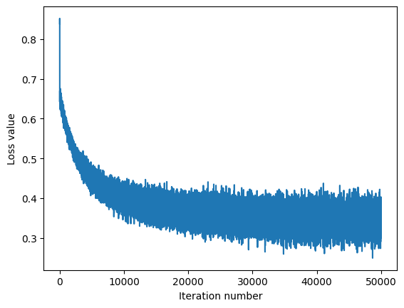
Plot the Loss

Plot the loss as a function of iteration number.

plt.plot(loss_hist)
plt.xlabel('Iteration number')
plt.ylabel('Loss value')
plt.show()

Test the Classifier

Evaluate the performance on both the training and validation set.

Y_train_pred = classifier.predict(X_train)
print('training accuracy: %f' % (np.mean(Y_train == Y_train_pred), ))
Y_test_pred = classifier.predict(X_test)
print('validation accuracy: %f' % (np.mean(y_test == Y_test_pred), ))

training accuracy: 0.852500
validation accuracy: 0.875000

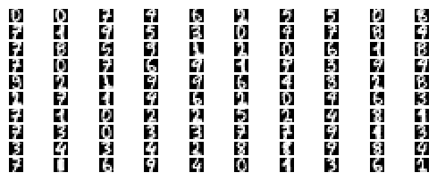
Handwritten Digits

This dataset is publicly available and can be downloaded from this link.

Training Data

data = np.loadtxt("./datasets/handwritten_digits/optdigits.tra", delimiter=",", dtype=int)
X_train = np.int32(data[:, 0:-1])  
Y_train = np.int32(data[:, -1]) 

print("Dimension numbers :", X_train.shape[1])
print("Number of data    :", X_train.shape[0])
print("Labels            :", np.unique(Y_train))

Dimension numbers : 64
Number of data    : 3823
Labels            : [0 1 2 3 4 5 6 7 8 9]

Test Data

data = np.loadtxt("./datasets/handwritten_digits/optdigits.tes", delimiter=",", dtype=int)
X_test = np.int32(data[:, 0:-1])  
Y_test = np.int32(data[:, -1]) 

print("Dimension numbers :", X_test.shape[1])
print("Number of data    :", X_test.shape[0])
print("Labels            :", np.unique(Y_test))

Dimension numbers : 64
Number of data    : 1797
Labels            : [0 1 2 3 4 5 6 7 8 9]

for i in range(100):
    X_train_ = X_train[i,:].reshape(8, 8)
    X_train_ = np.abs(255.0 - 255.0 / 16.0 * X_train_)
    plt.subplot(20, 10, i + 1)
    # Rescale the weights to be between 0 and 255
    plt.imshow(X_train_.astype('uint8'), cmap='Greys')
    plt.axis('off')

Train the Classifier

classifier = Softmax()
loss_hist = classifier.train(X_train, Y_train, learning_rate=1e-5, batch_size=None, num_iters=50000, verbose_step=10000)

iteration 0 / 50000: loss 2.309471

iteration 10000 / 50000: loss 0.798868

iteration 20000 / 50000: loss 0.690446

iteration 30000 / 50000: loss 0.669634

iteration 40000 / 50000: loss 0.663748

iteration 49999 / 50000: loss 0.661651

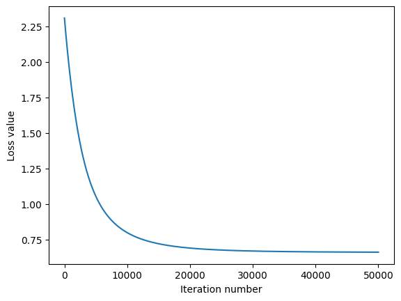
Plot the Loss

Plot the loss as a function of iteration number.

plt.plot(loss_hist)
plt.xlabel('Iteration number')
plt.ylabel('Loss value')
plt.show()

Test the Classifier

Evaluate the performance on both the training and validation set.

Y_train_pred = classifier.predict(X_train)
print('training accuracy: %f' % (np.mean(Y_train == Y_train_pred), ))
Y_test_pred = classifier.predict(X_test)
print('validation accuracy: %f' % (np.mean(Y_test == Y_test_pred), ))

training accuracy: 0.947423
validation accuracy: 0.922092

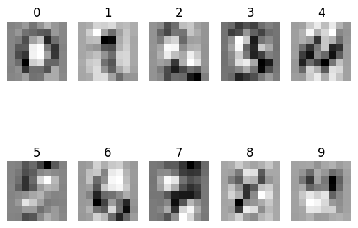
Visualize the Learned Weights

• Take matrix W and strip out the bias.

• For each class, reshape the matrix back into 2D arrays

• Plot the 2D arrays (matrices) as images.

w = classifier.W[:-1, :] # strip out the bias
w = w.reshape(8, 8, 10)
w_min, w_max = np.min(w), np.max(w)
classes = ['0', '1', '2', '3', '4', '5', '6', '7', '8', '9']

for i in range(10):
    plt.subplot(2, 5, i + 1)
      
    # Rescale the weights to be between 0 and 255
    wimg = 255.0 * (w[:, :, i].squeeze() - w_min) / (w_max - w_min)
    plt.imshow(wimg.astype('uint8'), cmap='Greys')
    plt.axis('off')
    plt.title(classes[i])