Dynamic Optimization

YADPF: Yet another Dynamic Programming Function A generic implementation of deterministic backward dynamic programming in MATLAB Auralius ManurungME - Universitas Pertamina Version 2021Table of Contents

1. Bertsekas' Two-Oven Problem 2. A Moving Mass (Double Integrator) 3. Optimal Storage Strategy (Single Integrator Problem) 4. Lotka-Volterra Fishery 5. Dubin's Car 6. Finding the Shortest Path on a Terrain 7. Sutton's Mountain Car 8. Two-Tank Problem 9. Piecewise Hanging Mass-Spring System 10. Time-Optimal van der Pol Equation with an Input 11. Time-Optimal Stabilization of an F8 Aircraft 12. References

Preface This current version of the notes is not yet complete. Please email me at auralius.manurung@ieee.org with any corrections or comments. 1. Bertsekas' Two-Oven Problem1A certain material is passed through a sequence of

N

ovens as shown in the figure below:

Drawing 1:The schematic of the two-oven problem.

Where:

x_{0}

: initial temperature of the material

x_{i}

: temperature of the material at the exit of oven

i

u_{i}

: prevailing temperature of oven

i

. The system's model is described as follows:

x_{k + 1} = (1 - a) x_{k} + a u_{k}, k = 0, 1

where

a

is a given scalar from the interval

(0, 1)

In order to keep the the final temperature

x_{2} = T

, the total incurring cost function is as follows:

J = r (x_{2} - T)^{2} + u_{0}^{2} + u_{1}^{2}

where

r

is any positive real number that will bring

x_{2}

close to

T

. Before we can apply dynamic programming algorithm to solve the two-oven problem above, we need to first formulate the problem in

(1)

and

(2)

into a more formal form, which is as follows:

\begin{array}{c} J_{N} = r (x_{N} - T)^{2} \\ J_{k} = J_{N} + \sum_{j = k}^{N - 1} u_{j}^{2}, N = 2, k = 0, \dots, N - 1 \end{array}

J_{2}^{*} = \begin{array}{c} \min \\ x_{2} \end{array} r (x_{2} - T)^{2}

J_{1}^{*} = \begin{array}{c} \min \\ u_{1} \end{array} [J_{2}^{*} + u_{1}^{2}]

J_{0}^{*} = \begin{array}{c} \min \\ u_{0}, u_{1} \end{array} [J_{2} + u_{1}^{2} + u_{0}^{2}] = \begin{array}{c} \min \\ u_{0} \end{array} [J_{1}^{*} + u_{0}^{2}]

The following computational grids are used for the dynamic programming algorithm implementation:

\begin{array}{c} x_{1}, x_{2} \in X_{k} (x_{k}) = {0, 1, \dots, 1000} \\ u_{k} \in U_{k} (u_{k}) = {0, 1, \dots, 1000} \end{array}

Here, we take

r = 100

a = 0.7

T = 300

, and

x_{0} = 30

. The optimization problem in

(3)

(6)

can actually be solved analytically. However, we will solve it numerically by using dynamic programming algorithm in YAPDF software package. The MATLAB implementation is shown in the code listing below. Besides the main function, we need to provide three other functions: state_update_fn, stage_cost_fn, and terminal_cost_fn. These three functions describe system dynamics, stage cost, and terminal cost, respectively. We must make sure that only element-wise operation occurs in these functions, especially for functions that work differently for matrices, such as: multiplication, power, exp, etc.

1% Initial and terminal states2x0 = 30;3xf = 300;4 5% Setup the states and the inputs6X = 0 : 0.1 : 1000;7U = 0 : 0.1 : 1000;8 9% Build the structure10dpf.states = {X};11dpf.inputs = {U};12dpf.T_ocp = 1;13dpf.T_dyn = 1;14dpf.n_horizon = 3;15dpf.state_update_fn = @state_update_fn;16dpf.stage_cost_fn = @stage_cost_fn;17dpf.terminal_cost_fn = @terminal_cost_fn;18 19% Initiate and run the solver, do forwar tracing and plot the results20dpf = yadpf_solve(dpf);21dpf = yadpf_trace(dpf, x0);22yadpf_plot(dpf, '-');23 24% Reachability plot25yadpf_rplot(dpf, xf, 10);26 27%% The state update function28function X = state_update_fn(X, U, ~)29a = 0.7;30X{1} = (1 - a).*X{1} + a * U{1};31end32 33%% The stage cost function34function J = stage_cost_fn(X, U, k, ~)35J = U{1}.^2;36end37 38%% The terminal cost function39function J = terminal_cost_fn(X)40xf = 300; % Desired terminal state41r = 1000; % Weighting factor42J = r * (X{1}-xf).^2;43end

The outputs of the above code listing are shown in the following Figure 1 and Figure 2. Notice that in YADPF, there are two sampling period: T_ocp and T_dyn. T_ocp is the sampling period for the optimal control problem (OCP) which defines the temporal discretization of the input. T_dyn is the sampling period for the dynamic simulation. T_dyn must be greater than or equal to T_ocp.

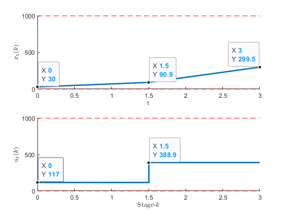
Figure 1:The optimal state and input variable for the two-oven problem

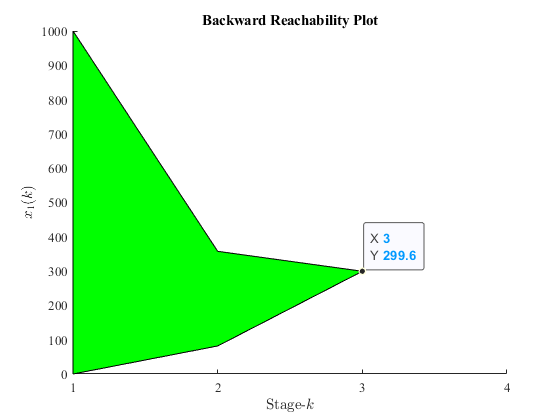
Figure 2:Backward reachability plot of the two-oven problem that shows all possible state evolution to reach a certain terminal condition.

2. A Moving Mass (Double Integrator)Given the following system:

Drawing 2:A mass-damper system is exposed to an external force.

Find an optimum set of

f

that brings

m

x_{f}

within

T_{f}

seconds. The desired terminal velocity is

v (T_{f}) = 0

and the constrain for

f

- 1 ⩽ f (t) ⩽ 1

. The equation of motion of the system described in the figure above is:

a (t) = \frac{f (t)}{m} - \frac{b}{m} v (t)

Rewriting

(7)

in its state space form:

[\begin{array}{c} v (t) \\ a (t) \end{array}] = [\begin{array}{cc} 0 & 1 \\ 0 & - \frac{b}{m} \end{array}] [\begin{array}{c} x (t) \\ v (t) \end{array}] + [\begin{array}{c} 0 \\ \frac{1}{m} \end{array}] g (t)

Discretizing

(8)

gives us:

[\begin{array}{c} v_{k + 1} \\ a_{k + 1} \end{array}] = [\begin{array}{cc} 1 & 𝛥 t \\ 0 & 1 - \frac{b}{m} 𝛥 t \end{array}] [\begin{array}{c} v_{k} \\ a_{k} \end{array}] + [\begin{array}{c} 0 \\ \frac{𝛥 t}{m} \end{array}] f_{k}

We define the following objective functions:• Minimization of the input

J_{1} = \sum_{k = 0}^{N - 1} f_{k}^{2}

• Minimization of the terminal position error

J_{2} = (x_{f} - x_{N})^{2}

• Minimization of the terminal velocity

J_{3} = (v_{f} - v_{N})^{2}

where

N

is the horizon length. The total objective function can then be written as:

J = 𝛼_{1} J_{1} + 𝛼_{2} J_{2} + 𝛼_{3} J_{3}

where

𝛼_{1}

𝛼_{2}

, and

𝛼_{3}

are any positive real numbers. Finally, the formulated problem is expressed as follows:

\begin{array}{c} \begin{array}{c} \min \\ f_{k} \\ k = 0, \dots, N - 1 \end{array} (𝛼_{1} \sum_{k = 0}^{N - 1} f_{k}^{2} + 𝛼_{2} (x_{f} - x_{N})^{2} + 𝛼_{3} (v_{f} - v_{N})^{2}) \\ such that: \\ [\begin{array}{c} v_{k + 1} \\ a_{k + 1} \end{array}] = [\begin{array}{cc} 1 & 𝛥 t \\ 0 & 1 - \frac{b}{m} 𝛥 t \end{array}] [\begin{array}{c} v_{k} \\ a_{k} \end{array}] + [\begin{array}{c} 0 \\ \frac{𝛥 t}{m} \end{array}] f_{k} \end{array}

An asterisk symbol represents an optimal value. To use dynamic programming to solve

(14)

, all states and inputs must be discretized first. Thus, we add more information to the problem and rewrite it as follows:

\begin{array}{c} \min \\ f_{k} \end{array} (𝛼_{1} \sum_{k = 0}^{N - 1} f (k)^{2} + 𝛼_{2} (x_{f} - x (N))^{2} + 𝛼_{3} (v_{f} - v (N))^{2})

such that:

\begin{array}{c} [\begin{array}{c} v_{k + 1} \\ a_{k + 1} \end{array}] = [\begin{array}{cc} 1 & 𝛥 t \\ 0 & 1 - \frac{b}{m} 𝛥 t \end{array}] [\begin{array}{c} v_{k} \\ a_{k} \end{array}] + [\begin{array}{c} 0 \\ \frac{𝛥 t}{m} \end{array}] f_{k} \\ f_{k} = F_{k} \in {- 4, - 3.9, - 3.8, \dots, 3.8, 3.9, 4} \\ x_{k} = X_{k} \in {0, 0.001, 0.002, \dots, 1} \\ v_{k} = V_{k} \in {0, 0.001, 0.002, \dots, 1} \end{array}

The following code listing shows the implementation of backward dynamic programming by using the YADPF.

1% Setup the states and the inputs2X = 0 : 0.001 : 1; % Position3V = 0 : 0.001 : 1; % Velocity4F = -4 : 0.1 : 4; % Applied force5 6% Setup the horizon7Tf = 1; % 1 second8T_ocp = 0.1; % Temporal discretization step9t = 0 : T_ocp : Tf;10 11dpf.states = {X, V};12dpf.inputs = {F};13dpf.T_ocp = T_ocp;14dpf.T_dyn = 0.01; % Time step for the dynamic simulation 15dpf.n_horizon = length(t);16dpf.state_update_fn = @state_update_fn;17dpf.stage_cost_fn = @stage_cost_fn;18dpf.terminal_cost_fn = @terminal_cost_fn;19 20% Initiate and run the solver, do forward tracing for the given initial 21% condition and plot the results22dpf = yadpf_solve(dpf);23dpf = yadpf_trace(dpf, [0 0]); % Initial state: [0 0]24yadpf_plot(dpf, '-');25 26% Optional: draw the reachability plot27yadpf_rplot(dpf, [0.5 0], 0.1);28 29%% The state unpdate funtion 30function X = state_update_fn(X, F, dt)31m = 1; % Mass32b = 0.1; % Damping coefficient33 34X{1} = X{1} + dt*X{2};35X{2} = X{2} - b/m*dt.*X{2} + dt/m.*F{1};36end37 38%% The stage cost function39function J = stage_cost_fn(X, F, k, dt)40J = dt*F{1}.^2;41end42 43%% The terminal cost function44function J = terminal_cost_fn(X)45xf = [0.5 0];46 47% Control gains48r1 = 1000;49r2 = 100;50 51J = r1*(X{1}-xf(1)).^2 + r2*(X{2}-xf(2)).^2;52end

The results are shown as follows:

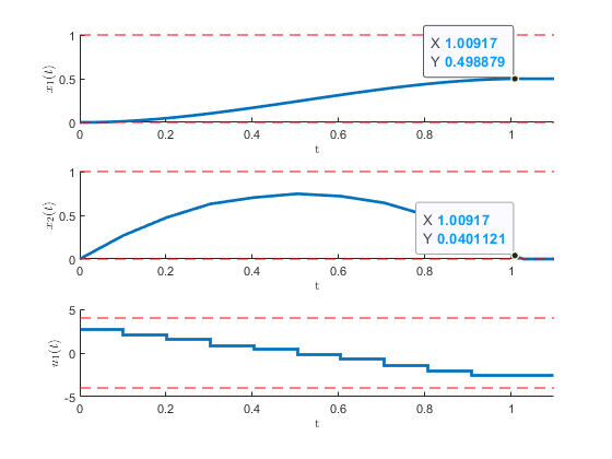
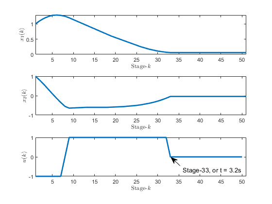
Figure 3:The optimal states and input for the mass-damper optimal control problem.

3. Optimal Storage Strategy (Single Integrator Problem)This example is taken from

(Jonsson, 2010)

. The stock grow equation is defined as follows:

\dot{x} (t) = u (t), x (0) = 0

where

x

is the stock size and

u

is the production rate. The goal is to have at least

A

units of commodity in storage at some prescribed time

t_{f}

. This goal should be obtained at minimum cost. If we let

r

be production cost growth rate and

c

storage cost per time unit, then the total cost becomes:

J = \int_{0}^{t_{f}} (u_{k} e^{r t} + c x (t)) d t

In discrete form, the optimal control problem can be written as follows:

\begin{array}{c} \begin{array}{c} \min \\ u_{k} \end{array} \underset{Stage cost}{\underset{⏟}{\sum_{k = 0}^{N - 1} (u_{k} e^{r k T_{s}} + c x_{k}) T_{s}}} + \underset{Terminal cost}{\underset{⏟}{L (x_{N} - A)^{2}}} \\ such that \\ x (k + 1) = u (k) T_{s} + u_{k} \\ x_{k} = X_{k} \in {0, 0.1, \dots, 500} \\ u_{k} = U_{k} \in {0, 0.1, \dots, 10} \end{array}

Let us define

r = 0.1

c = 10

T_{s} = 1

A = 200

, and

L = 100

. Additionally, notice that we add an additional terminal cost in

(18)

in order to meet the desired terminal state. Initially we set

x_{0} = 0

. Now, let us use the reusable dynamic programming algorithm function provided in YADPF.

1% Setup the states and the inputs2X = 0 : 0.1 : 500;3U = 0 : 0.1 : 10;4 5% Setup the horizon6T_ocp = 1; % Every 1 day7T_vect = 0 : T_ocp : 30; % Day-0 to day-308 9x0 = 0; % Initial state10xf = 200; % Terminal state11 12dpf.states = {X};13dpf.inputs = {U};14dpf.T_ocp = T_ocp;15dpf.T_dyn = T_ocp;16dpf.n_horizon = n_horizon;17dpf.state_update_fn = @state_update_fn;18dpf.stage_cost_fn = @stage_cost_fn;19dpf.terminal_cost_fn = @terminal_cost_fn;20 21% Initiate and run the solver, do forwar tracing and plot the results22dpf = yadpf_solve(dpf);23dpf = yadpf_trace(dpf, x0);24yadpf_plot(dpf, '-d');25 26% Reachability plot27yadpf_rplot(dpf, xf, 10);28 29%% State update function30function X = state_update_fn(X, U, dt)31X{1} = dt*U{1} + X{1}; 32end33 34%% Stage cost function35function J = stage_cost_fn(X, U, k, dt)36r = 0.1; % production cost growth rate37c = 10; % storage cost per time unit38J = dt*exp(r*k*dt)*U{1} + c*X{1}*dt;39end40 41%% Terminal cost function42function J = terminal_cost_fn(X)43xf = 200; 44L = 100;45J = L .* (xf-X{1}).^2;46end

Running the code listing above gives us the following results.

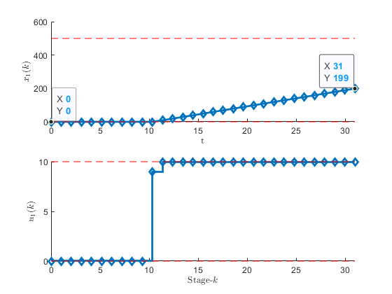
Figure 4:The optimization results for the optimal storage strategy problem.

When the state variable is part of the cost function, our problem becomes a time optimal control problem. This is because whenever the state variable is non-zero, the cost is increased. Thus, it makes sense to delay the production such that we meet the terminal state at the end of the horizon. Since it is a time-optimal control problem, we notice that there is a bang-bang action in the control input. The control input is switched to its allowable maximum value.

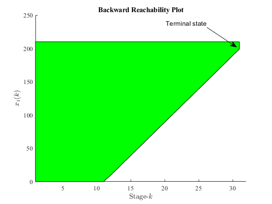
Figure 5:Backward reachability plot of a targeted terminal state.

4. Lotka-Volterra FisheryThis problem is taken from

(Sundstrom & Guzzella, 2009)

, with some modifications. Given the following discrete dynamic system:

x_{k + 1} = f (x_{k}, u_{k}) + x_{k}, k = 0, 1, \dots, N - 1

where

f (x_{k}, u_{k}) = T_{s} (\frac{2}{100} (x_{k} - \frac{x_{k}^{2}}{1000}) - u_{k})

where

N

is the horizon length,

x_{k}

is the amount of fishes in the lake and

u_{k}

is the fishing rate. Time unit is in "days". The time horizon is set to 200 days with a sampling of

T_{s} = 0.5

days. The goal is to maximize the amount of fishes caught over a fixed period of time. By he 200th day, at least 750 fish are still in the lake. Thus, the following objective function is used:

J = \sum_{k = 1}^{N - 1} (- u_{k})

Let us reformulate the problem above as follow:

\begin{array}{c} \begin{array}{c} \min \\ u_{k} \end{array} {\sum_{k = 1}^{N - 1} (- u_{k})} \\ such that: \\ x_{k + 1} = T_{s} (\frac{2}{100} (x_{k} - \frac{x_{k}^{2}}{1000}) - u_{k}) + x_{k} \\ x_{k} \in {0, 1, \dots, 1000} \\ u_{k} \in {0, 0.1, 1, \dots, 10} \end{array}

MATLAB implementation of

(22)

by using YADPF is as follows.

% Initial and terminal statex0 = 250;xf = 750; % Setup the states and the inputsX = 0 : 0.1 : 1000;U = 0 : 1 : 10; % Setup the horizonTf = 200; % 200 daysT_ocp = 0.2; % Every half dayt = 0 : T_ocp : Tf; dpf.states = {X};dpf.inputs = {U};dpf.T_ocp = T_ocp;dpf.T_dyn = 0.01;dpf.n_horizon = length(t);dpf.state_update_fn = @state_update_fn;dpf.stage_cost_fn = @stage_cost_fn;dpf.terminal_cost_fn = @terminal_cost_fn; % Initiate and run the solver, do forward tracing and plot the resultsdpf = yadpf_solve(dpf);dpf = yadpf_trace(dpf, x0);yadpf_plot(dpf, '-'); % Draw the reachability plotyadpf_rplot(dpf, xf, 5); %% The state update functionfunction X = state_update_fn(X, U, dt)X{1} = X{1} + dt * (0.02 * (X{1}-X{1}.^2./ 1000) - U{1});end %% The stage cost functionfunction J = stage_cost_fn(X, U, k, dt)J = -dt .* U{1};end %% The terminal cost functionfunction J = terminal_cost_fn(X)xf = 750; % Terminal stater = 1000;J = r * (xf-X{1}).^2;end

The optimization results are shown in the following figures.

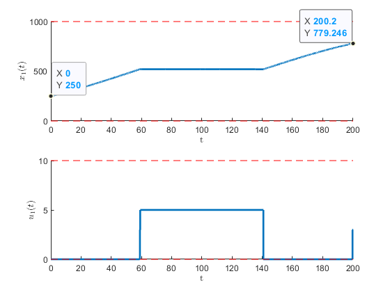
Figure 6:The optimal input and the resulting state values for the Lotka-Volterra fishery problem generated by the dynamic programming.

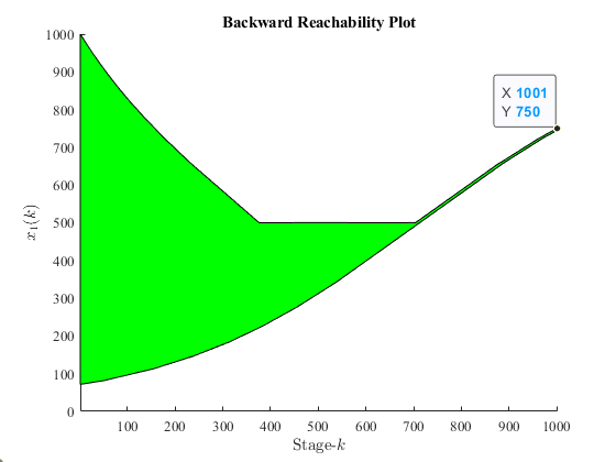
Figure 7:The reachable and unreachable states for the Lotka-Volterra fishery problem in order to reach a given terminal state.

5. Dubin's Car The kinematics of a car is described by the following differential equations:

\begin{aligned} \dot{x} (t) & = v \cos (𝜃 (t)) \\ \dot{y} (t) & = v \sin (𝜃 (t)) \\ \dot{𝜃} (t) & = 𝜔 (t) \end{aligned}

where: •

𝜔

is the angular velocity of the car and

| 𝜔 | \leq v / R

•

R

is the lower bound for the turning radius•

(x, y)

are the coordinates of the reference point of the car•

𝜃

is the direction (heading) of the car• and

v

is the constant speed of the car

Drawing 3:Schematic and parameters of a Dubins' car

Find the optimum path from a given initial point to a terminal point. The car must arrive at the terminal point at time

t_{f}

. Thus, the objective function is defined as:

J = \sum_{k = 0}^{N - 1} 𝜔_{k}^{2} + (x_{N} - A)^{2} + (y_{N} - B)^{2} + (𝜃_{N} - C)^{2}

Discretizing

(23)

gives us:

\begin{aligned} x_{k + 1} & = T_{s} v \cos (𝜃_{k}) + x_{k} \\ y_{k + 1} & = T_{s} v \sin (𝜃_{k}) + y_{k} \\ 𝜃_{k + 1} & = T_{s} 𝜔_{k} + 𝜃_{k} \end{aligned}

In the Dubin's car problem, typically we are looking for a time optimal solution. On the other hand, backward dynamic programming has a predefined fixed horizon. Thus, we must reach the terminal state before the final horizon and stop updating the state variables as soon as the terminal state is reached. However, in the Dubin's car problem, the car has constant speed and it can not stop. In order to implement the Dubin's car problem in MATLAB by using YAPDF, we formalize the problem as follows:

\begin{array}{c} \begin{array}{c} \min \\ 𝜔_{k} \in 𝛺_{k} \end{array} \sum_{k = 0}^{N - 1} 𝜔_{k}^{2} + (x_{N} - A)^{2} + (y_{N} - B)^{2} + (𝜃_{N} - C)^{2} \\ such that \\ \begin{aligned} x_{k + 1} & = T_{s} v \cos (𝜃_{k}) + x_{k} \\ y_{k + 1} & = T_{s} v \sin (𝜃_{k}) + y_{k} \\ 𝜃_{k + 1} & = T_{s} 𝜔_{k} + 𝜃_{k} \\ x_{k} & \in X_{k} \\ y_{k} & \in Y_{k} \\ 𝜃_{k} & \in 𝛩_{k} \\ 𝜔 & \in 𝛺_{k} \end{aligned} \end{array}

Taking a case where the car is the initially located at

[0, 0, 0]

and is moving to terminal as

[0, 0, - 2 𝜋]

. we then define the following discrete world:

\begin{aligned} X_{k} & = {- 1, - 0.09, \dots, 1} \\ Y_{k} & = {- 1, - 0.99, \dots, 0} \\ 𝛩_{k} & = {- 2 𝜋, - 2 𝜋 + 0.01, \dots, 0} \\ 𝛺_{k} & = {- \frac{v}{R}, 0, \frac{v}{R}} \end{aligned}

Let us take

v = 1

and

R = 0.5

. The MATLAB implementation of

(26)

with YADPF is as follows.

1global v xf;2 3% Define the Dubin's car parameters4R = 0.5; % lower bound for the turning radius5v = 1; % the constant speed of the car 6 7% Setup the states and the inputs8X = -1 : 0.01 : 1;9Y = -1 : 0.01 : 0;10THETA = -2*pi : 0.01 : 0;11OMEGA = [-v/R 0 v/R];12 13% Setup the horizon14T_ocp = 0.2; % Temporal discretization step15Tf = pi; % Theoritical completion time, otherwise the car will go around-and-around16t = 0 : T_ocp : Tf;17 18% Initial and terminal states19% We are going to make a full cricle of radius R20x0 = [0 0 0];21xf = [0 0 -2*pi];22 23% Build the structure24dpf.states = {X, Y, THETA};25dpf.inputs = {OMEGA};26dpf.T_ocp = T_ocp;27dpf.T_dyn = 0.01;28dpf.n_horizon = length(t);29dpf.state_update_fn = @state_update_fn;30dpf.stage_cost_fn = @stage_cost_fn;31dpf.terminal_cost_fn = @terminal_cost_fn;32 33% Initiate and run the solver, do forwar tracing and plot the results34dpf = yadpf_solve(dpf);35dpf = yadpf_trace(dpf, x0);36yadpf_plot(dpf, '-');37 38% Animation39visualize(dpf);40 41%% The state update function42function X = state_update_fn(X, U, dt)43global v;44 45% X{1} is x, X{2} is y, and X{3} is theta, and U is omega46X{1} = dt*v*cos(X{3})+X{1};47X{2} = dt*v*sin(X{3})+X{2};48X{3} = dt*v*U{1}+X{3};49end50 51%% The stage cost function52function J = stage_cost_fn(X, U, k, dt)53J = dt * U{1}.^2; % Minimize the input54end55 56%% The terminal cost function57function J = terminal_cost_fn(X)58global xf;59% Weighting factors60r = 1000;61 62% Calculate the cost63J = r*(X{1}-xf(1)).^2 + r*(X{2}-xf(2)).^2 + r*(X{3}-xf(3)).^2;64end65 66%% Animate the car's motion in XY-space67function visualize(dpf)68% Please rsee the provided repository.69end

The results are shown in Figure 8 and Figure 9 below.

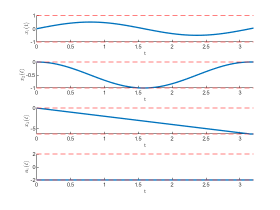
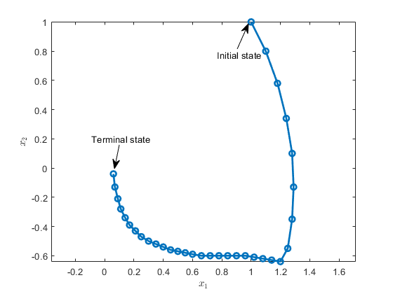
Figure 8:Optimal state evolution of the Dubin's car which is located at

[0, 0, 0]

and moving to terminal as

[0, 0, - 2 𝜋]

Figure 9: Optimal path for the car, which is initially located at

[0, 0, 0]

and moving to terminal as

[0, 0, - 2 𝜋]

6. Finding the Shortest Path on a TerrainA car is positioned

x_{0}, y_{0}

. The motion of the car is entirely kinematic and is given as follows:

\begin{array}{c} x_{k + 1} = x_{k} + u_{k} \\ y_{k + 1} = y_{k} + v_{k} \end{array}

where

u_{k}

and

v_{k}

are defined as follows:

\begin{array}{c} u_{k} \in {- 1, 0, 1} \\ v_{k} \in {- 1, 0, 1} \end{array}

Thus, the car can only move one grid per stage.

Drawing 4:A kinematic cat that can only move one grit at a time

When applying input

u

and

v

, the following rules apply.• When

u = 1, v = 0

, the car moves right.• When

u = - 1, v = 0

, the car moves left.• When

u = 0, v = 1

, the car moves up.• When

u = 0, v = - 1

, the car moves down. The objective function here is to travel as close as possible to the target coordinate

(x_{T}, y_{T})

. The travel time should be as short as possible. During the travel, the car must avoid the climb trajectories. However, the descent trajectories does not benefit the car either. Thus, descent trajectories are not more preferable than flat trajectories. Mathematically, the objective function is defined as follows:

J^{*} = \begin{array}{c} \min \\ u_{k} \end{array} {𝛼 (x_{T} - x_{N})^{2} + 𝛼 (y_{T} - y_{N})^{2} + \sum_{k + 0}^{N - 1} [u_{k}^{2} + v_{k}^{2} + 𝛽 𝛥 h_{k} (u_{k})]}

where

𝛥 h_{k} (u_{k}) = \max (z_{k + 1} - z_{k}, 0)

, which represents the height difference when a certain

u_{k}

is applied. However, when the height difference is negative,

𝛥 h

is set to

0

r

is the control gain that regulates the terminal position of the car. As a result, we can write down the optimal control problem as follows:

\begin{array}{c} \begin{array}{c} \min \\ u_{k} \end{array} {𝛼 (x_{T} - x_{N})^{2} + 𝛼 (y_{T} - y_{N})^{2} + \sum_{k + 0}^{N - 1} [u_{k}^{2} + v_{k}^{2} + 𝛽 𝛥 h_{k} (u_{k})]} \\ such that: \\ x_{k + 1} = x_{k} + u_{k} \\ y_{k + 1} = y_{k} + v_{k} \\ u_{k} \in {- 1, 0, 1} \\ v_{k} \in {- 1, 0, 1} \end{array}

MATLAB implementation by using YADPF of

(31)

is as follows. First, a MAT file containing a square matrix is provided. Matrix element at row number

m

and column number

n

is the terrain height at coordinate

(m, n)

. This height matrix is generated by another MATLAB function that can be found in this link2

global T terra_size; % Terrain1.mat, from 1 to 4225 (64x64)% Terrain2.mat, from 1 to 16641 (129x129)load ('Terrain1.mat');%load ('Terrain2.mat');terra_size = size(T); % Setup the states and the inputsX = 1 : 1 : length(T);Y = 1 : 1 : length(T);Ux = [-1 0 1];Uy = [-1 0 1]; % Prepare the structuredpf.states = {X, Y};dpf.inputs = {Ux Uy};dpf.T_ocp = 1;dpf.T_dyn = 1;dpf.n_horizon = 150;dpf.state_update_fn = @state_update_fn;dpf.stage_cost_fn = @stage_cost_fn;dpf.terminal_cost_fn = @terminal_cost_fn; % Initiate and run the solver, do forwar tracing and plot the resultsdpf = yadpf_solve(dpf);dpf = yadpf_trace(dpf, [1 1]); % Initial state: [1 1]yadpf_plot(dpf, '-'); % Additional plottingfigurehold onsurf(T');plot3(dpf.x_star{1}, dpf.x_star{2}, T(sub2ind(terra_size, ... dpf.x_star{1}, dpf.x_star{2})), '-r', 'LineWidth',2);view([-46.1 49.7]);xlabel('x')ylabel('y')axis equal %% The state update functionfunction X = state_update_fn(X, U, ~)X{1} = X{1} + U{1};X{2} = X{2} + U{2};end %% The stage cost functionfunction J = stage_cost_fn(X, U, k, ~)global terra_size; r = terra_size(1);c = terra_size(2); % First, check where the car's next position for a selected inputX_to = state_update_fn(X, U);X_to{1} = min(max(X_to{1},1),r);X_to{2} = min(max(X_to{2},1),c); % Next, compute the height difference of the current position to the next% positiondh = get_height_difference(X{1}, X{2}, X_to{1}, X_to{2}); % Finally, compute the costw = 2;J = U{1}.^2 + U{2}.^2 + w.*max(dh,0);end %% The terminal cost functionfunction J = terminal_cost_fn(X)% Weighting factorsk1 = 100;k2 = 100; % Final statesxf = [50 60]; J = k1*(X{1}-xf(1)).^2 + k2.*(X{2}-xf(2)).^2;end %% This function computes the height differece between two location % coordinatesfunction dh = get_height_difference(x_from, y_from, x_to, y_to)global T terra_size; r = terra_size(1);c = terra_size(2); to_id = sub2ind([r c], x_to, y_to);from_id = sub2ind([r c], x_from, y_from); dh = T(to_id) - T(from_id);end

It can be seen from the listing above that before we can compute the stage cost, we must first compute the height difference of the current position coordinate to the next position coordinate for every possible input combination. Thus, we add a new function: get_height_difference. The outputs from the code listing above are given in Figure 10 and Figure 11.

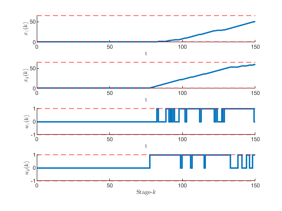
Figure 10:State evolution and control input sequence for a given initial position to a targeted terminal position

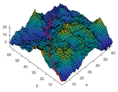
Figure 11:An example of an optimal path found by the dynamic programming algorithm

7. Sutton's Mountain CarThere are many variations of the mountain car problems. The mountain car problem that we will solve here is taken from a popular text book authored by Sutton and Barto

(Sutton & Barto, 2018)

. The problem is stated as follows (with necessary modifications): Consider the task of driving an under-powered car up a steep mountain road. The difficulty is that gravity is stronger than the car’s engine, and even at full throttle the car cannot accelerate up the steep slope. The only solution is to first move away from the goal and up the opposite slope on the left. Then, by applying full throttle the car can build up enough inertia to carry it up the steep slope even though it is slowing down the whole way. This is a simple example of a continuous control task where things have to get worse in a sense (farther from the goal) before they can get better. Many control methodologies have great difficulties with tasks of this kind unless explicitly aided by a human designer.

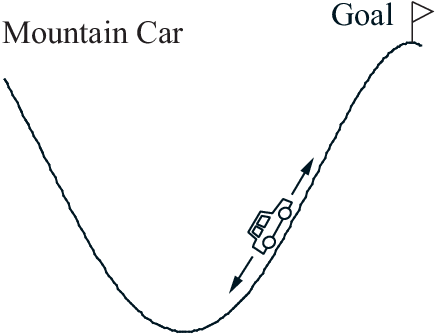
Figure 12:The Sutton's mountain car problem

The reward in this problem is 1 on all time steps until the car moves past its goal position at the top of the mountain, which ends the episode. There are three possible actions: full throttle forward (+1), full throttle reverse (-1), and zero throttle (0). The car moves according to a simplified physics. Its position,

x_{k}

, and velocity,

{\dot{x}}_{k}

, are updated by:

\begin{aligned} x_{k + 1} = bound [x_{k} + {\dot{x}}_{k + 1}] \\ {\dot{x}}_{k + 1} = bound [{\dot{x}}_{k} + 0.001 A_{k} - 0.0025 \cos (3 x_{k})] \end{aligned}

where the bound operation enforces

- 1.2 ⩽ x_{k} ⩽ 0.5

and

- 0.07 ⩽ {\dot{x}}_{k} ⩽ 0.07

. In addition, when

x_{k}

reached the left bound,

{\dot{x}}_{k}

was reset to zero. When it reached the right bound, the goal was reached and the episode was terminated. Each episode started from a random position

x_{0} \in [- 0.6, - 0.4]

and zero velocity. To solve the problem above, we start by formalizing it as follows:

\begin{array}{c} \begin{array}{c} \min \\ u_{k} \end{array} {u_{k}^{2} + (x_{N} - 0.5)^{2} + {\dot{x}}_{N}}, k = 0, 2, \dots, N - 1 \\ such that: \\ x_{k + 1} = x_{k} + {\dot{x}}_{k + 1} \\ {\dot{x}}_{k + 1} = {\dot{x}}_{k} + 0.001 A_{k} - 0.0025 \cos (3 x_{k}) \\ x_{k} \in {- 1.2, - 1.199, \dots, 0.5} \\ {\dot{x}}_{k} \in {- 0.07, - 0.069, \dots, 0.07} \end{array}

MATLAB implementation of

(33)

by using YADPF is as follows.

% Setup the states and the inputsP = -1.2 : 0.001 : 0.5;V = -0.07 : 0.0001 : 0.07;U = [-1 0 1]; dpf.states = {P V};dpf.inputs = {U};dpf.T_ocp = 1;dpf.T_dyn = 1;dpf.n_horizon = 140;dpf.state_update_fn = @state_update_fn;dpf.stage_cost_fn = @stage_cost_fn;dpf.terminal_cost_fn = @terminal_cost_fn; % Initiate and run the solver, do forwar tracing and plot the resultsdpf = yadpf_solve(dpf);dpf = yadpf_trace(dpf, [-0.5 0]); % Initial state: [-0.5 0]yadpf_plot(dpf, '-'); % Animate the mountatin carvisualize(dpf); % Draw the reachability plot, this may take quite some time% yadpf_rplot(dpf, [0.5 0], 0.1); %% The state update functionfunction X = state_update_fn(X, U, ~)X{2} = X{2} + 0.001*U{1} - 0.0025*cos(3*X{1});X{1} = X{1} + X{2}; % Hitting the left wall[r,c] = find(X{1}(:,:) <= -1.2);X{2}(r,c) = 0.001; % Inelastic wallend %% The stage cost function function J = stage_cost_fn(X, U, k, ~)xf = [0.5 0]; % Terminal state r1 = 1000;r2 = 1000;r3 = 5; J = r1*(X{1}-xf(1)).^2 + r2*(X{2}-xf(2)).^2 + r3*U{1}.^2;end %% The terminal cost function function J = terminal_cost_fn(X)xf = [0.5 0]; % Terminal state r1 = 1000;r2 = 1000; J = r1*(X{1}-xf(1)).^2 + r2*(X{2}-xf(2)).^2;end %% -----------------------------------------------------------------------function visualize(dpf)% Please see the complete codes in the provided repository.end

The results are presented in Figure 13 and Figure 14.Initially, we do not know the shortest possible time for the car to complete task. Thus, we guess the completion time by initially setting the horizon to

200

. However, the car manage to finish the task before the final horizon. The results are shown in Figure 13 and Figure 14.

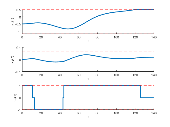
Figure 13:State evolution and control input sequence of the mountain car

Figure 14:Animation of the car's optimal movement

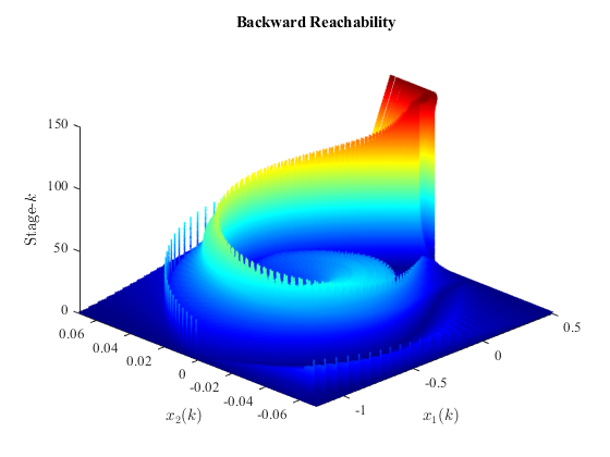
Figure 15:Reachability plot of the Sutton's mountain car's problem.

8. Two-Tank ProblemThe two tank problem is taken from

(Elbert et al., 2013)

. The task here is to fill both tanks within time

t_{f}

. The input

u_{1}

commands total water flows. The input

u_{2}

commands the water flow distribution between the two tanks. The values for these inputs are from

0

1

. When

u_{2} = 0.5

, same amount of water flows to both tanks. Both tanks have leaks that are proportional to the amount of water in the tank. The volume of the tanks (

x_{1}

and

x_{2}

) are also from

0

1

Drawing 5:Illustration of the two tank problem

The dynamics of the system is governed by the following equations.

\begin{aligned} {\dot{x}}_{1} (t) = & - \frac{1}{2} x_{1} (t) + u_{1} (t) u_{2} (t) \\ {\dot{x}}_{2} (t) = & - \frac{1}{2} x_{2} (t) + u_{1} (t) (1 - u_{2} (t)) \end{aligned}

Our goal is to fill the tank such that after two seconds, both tanks are half full. For this purpose, the cost function is given as follows.

J = \int_{0}^{t_{f}} u_{1} (t) + 0.1 | u_{2} (t) - 0.5 | d t

where

t_{f} = 2

. we start by formalizing

(34)

and

(35)

into an optimal control problem as follows.

\begin{array}{c} \begin{array}{c} \min \\ u_{k} \end{array} \sum_{k = 0}^{N - 1} {u_{1}^{k} + 0.1 | u_{2}^{k} - 0.5 |} \\ such that \\ \begin{aligned} x_{1}^{k + 1} = & T_{s} (- \frac{1}{2} x_{1}^{k} + u_{1}^{k} u_{2}^{k}) + x_{1}^{k} \\ x_{2}^{k + 1} = & T_{s} (- \frac{1}{2} x_{2}^{k} + u_{1}^{k} (1 - u_{2}^{k})) + x_{2}^{k} \\ u_{1}^{k} \in & U_{1}^{k} \\ u_{2}^{k} \in & U_{2}^{k} \\ x_{1}^{k} \in & X_{1}^{k} \\ x_{2}^{k} \in & X_{2}^{k} \end{aligned} \end{array}

9. Piecewise Hanging Mass-Spring SystemOur task here is to find the equilibrium position of a mass-spring system hanging from two anchor points as shown in Drawing 6. This problem is similar to the problem that can be found in this MATLAB documentation page . However, we will address the problem by using the dynamic optimization method.

Drawing 6:Hanging piecewise linear spring due to the gravity

To turn the problem above into an dynamic optimization problem, let us consider a planar kinematic car which is initially located at anchor 1. The car takes two vectors as its input:

u_{x}

and

u_{y}

. The resulting motion of the car is given the by the sum of these two vectors. The car must arrive at anchor 2 within six stages (number of horizons:

N + 1 = 7

). The dynamic of the car is governed by the following equations.

\begin{aligned} x_{k + 1} & = x_{k} + u_{x}^{k} \\ y_{k + 1} & = y_{k} + u_{y}^{k} \end{aligned}

Let us take the location of

m_{i}

(x_{i}, y_{i})

and the normal length of spring-

i

l_{i}

. The potential energy caused by the spring-

i

can be written as:

T_{i} = \frac{1}{2} k_{i} (\sqrt{(x_{i} - x_{i - 1})^{2} + (y_{i} - y_{i - 1})^{2}} - l_{i})^{2}

While the energy caused by the gravity can be written as:

V_{i} = m_{i} g x_{i}

Thus, the total energy is considered as cost that must be minimized. It is described as follows:

J = \sum_{i = 0}^{5} (T_{i} + V_{i}) + R (x_{6} - A)^{2} + R (y_{6} - B)^{2}

Drawing 7:Analogous planar kinematic car to model the piecewise linear springs

	MATLAB Cone Method	DPA-1Grind Size: $0.05$	DPA-2Grid Size: $0.03$
Anchor 1	$[0, 5]$	$[0, 5]$	$[0, 5]$
Spring 1	$[0.8476, 2.8835]$	$[0.65, 2.9]$	$[0.81, 2.85]$
Spring 2	$[1.3675, 2.1207]$	$[1.25, 2.15]$	$[1.32, 2.07]$
Spring 3	$[2.2506, 1.2789$	$[2.15, 1.3]$	$[2.16, 1.17]$
Spring 4	$[4.0897, 2.3711]$	$[3.95, 2.5]$	$[3.99, 2.34]$
Spring 5	$[4.7089, 3.3774]$	$[4.65, 3.45]$	$[4.59, 3.39]$
Anchor 2 / Spring 6	$[5, 4]$	$[5, 4]$	$[5, 4]$

10. Time-Optimal van der Pol Equation with an Input

11. Time-Optimal Stabilization of an F8 Aircraft

12. References

Bertsekas, D. P. (2000). Dynamic Programming and Optimal Control (2nd ed.). Athena Scientific.

Elbert, P., Ebbesen, S., & Guzzella, L. (2013). Implementation of dynamic programming for n-dimensional optimal control problems with final state constraints. IEEE Transactions on Control Systems Technology, 21(3), 924–931.

Jonsson, U. (2010). Optimal Control. Optimization and Systems Theory, KTH.

Miretti, F., Misul, D., & Spessa, E. (2021). DynaProg: Deterministic Dynamic Programming solver for finite horizon multi-stage decision problems. SoftwareX, 14, 100690.

Sundstrom, O., & Guzzella, L. (2009). A Generic Dynamic Programming Matlab Function. 18th IEEE International Conference on Control Applications, 7, 1625–1630.

Sutton, R. S., & Barto, A. G. (2018). Reinforcement Learning: An Introduction (2nd ed.). The MIT Press.

https://ocw.mit.edu/courses/electrical-engineering-and-computer-science/6-231-dynamic-programming-and-stochastic-control-fall-2015/lecture-notes/MIT6_231F15_Lec2.pdf

http://knight.temple.edu/~lakaemper/courses/cis350_2004/assignments/assignment_02.htm

␒x(t)	=vcos(𝜃(t))
␒y(t)	=vsin(𝜃(t))
␒𝜃(t)	=𝜔(t)

xk+1	=Ts vcos(𝜃k)+xk
yk+1	=Ts vsin(𝜃k)+yk
𝜃k+1	=Ts 𝜔k+𝜃k

xk+1	=Ts vcos(𝜃k)+xk
yk+1	=Ts vsin(𝜃k)+yk
𝜃k+1	=Ts 𝜔k+𝜃k
xk	∈Xk
yk	∈Yk
𝜃k	∈𝛩k
𝜔	∈𝛺k

Xk	={-1,-0.09,…,1}
Yk	={-1,-0.99,…,0}
𝛩k	={-2𝜋,-2𝜋+0.01,…,0}
𝛺k	={-v R,0,v R}

␒x1(t)=	-1 2x1(t)+u1(t)u2(t)
␒x2(t)=	-1 2x2(t)+u1(t)(1-u2(t))

	xk+1= bound [xk+␒xk+1]
	␒xk+1= bound [␒xk+0.001Ak-0.0025cos(3xk)]

xk+11=	Ts(-1 2xk1+uk1uk2)+xk1
xk+12=	Ts(-1 2xk2+uk1(1-uk2))+xk2
uk1∈	Uk1
uk2∈	Uk2
xk1∈	Xk1
xk2∈	Xk2

1	𝛥t
0	1-b m𝛥t

1	𝛥t
0	1-b m𝛥t

1	𝛥t
0	1-b m𝛥t

xk+1	=xk+ukx
yk+1	=yk+uky