Principle Component Analysis
This document is based on: Principal Component Analysis from Scratch
There are some differences:
svd decomposition of the covariance matrix is used instead of the Eigen decomposition. Thus, the Eigen value and vector pairs are always in non-ascending order.
Additional Eigen value correction is an optional step which is needed to obtain identical results with scikit-learn.
What is PCA?
Greenacre, M., Groenen, P.J.F., Hastie, T. et al. Principal component analysis. Nat Rev Methods Primers 2, 100 (2022):
PCA reduces a cases-by-variables data table to its essential features, called principal components.
Principal components are a few linear combinations of the original variables that maximally explain the variance of all the variables.
The method provides an approximation of the original data table using only these few major components.
Preparations
import numpy as np
import matplotlib.pyplot as plt

plt.rcParams.update({
    "text.usetex": False,
    "font.family": "sans-serif",
    "font.size": 8,
})

np.set_printoptions(precision=3, suppress=True)
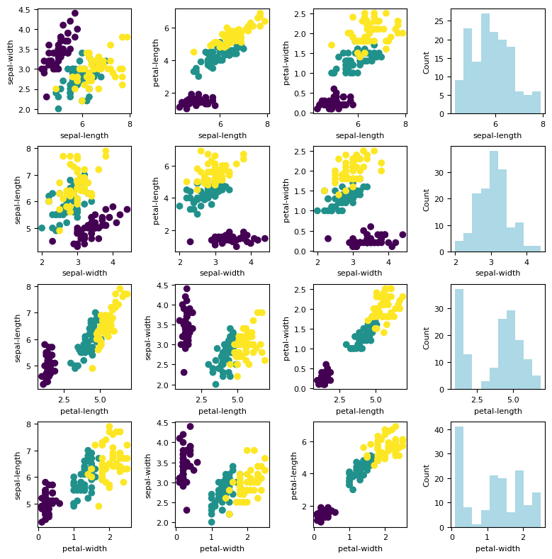
Iris Dataset
The iris data is ideal for our learning purpose since the data has only 4 features: sepal-length, sepal-width, petal-length, and petal-width.
More information about iris plan can be found here this Wikipedia link.
Load the Dataset
data = np.loadtxt("./datasets/iris/iris.data", delimiter=",", dtype=str)
X = np.float32(data[:, 0:4])  # 4 features

# Change the labels: string labels to numerical labels:
# Iris-setosa     = 0
# Iris-versicolor = 1
# Iris-virginica  = 2
y = np.zeros(X.shape[0], dtype=np.int32)
y[np.where(data[:,-1]=='Iris-setosa')]     = 0
y[np.where(data[:,-1]=='Iris-versicolor')] = 1
y[np.where(data[:,-1]=='Iris-virginica')]  = 2

feature_names = ['sepal-length', 'sepal-width', 'petal-length', 'petal-width']
n_features = X.shape[1]

print("Feature numbers :", X.shape[1])
print("Number of data  :", X.shape[0])
print("Labels          :", np.unique(y))
Feature numbers : 4
Number of data  : 150
Labels          : [0 1 2]
%matplotlib inline

fig, ax = plt.subplots(nrows=n_features, ncols=n_features, figsize= (n_features*2, n_features*2))
fig.tight_layout(pad=2.0)

names = feature_names

for i in range(n_features):
    J = np.arange(n_features)
    J = np.delete(J, i)
    for k, j in enumerate(J):
        ax[i, k].scatter(X[:, i], X[:, j], c = y)
        ax[i, k].set_xlabel(names[i])
        ax[i, k].set_ylabel(names[j])

for i in range(n_features):
    ax[i, -1].hist(X[:, i], color = 'lightblue')
    ax[i, -1].set_ylabel('Count')
    ax[i, -1].set_xlabel(names[i])
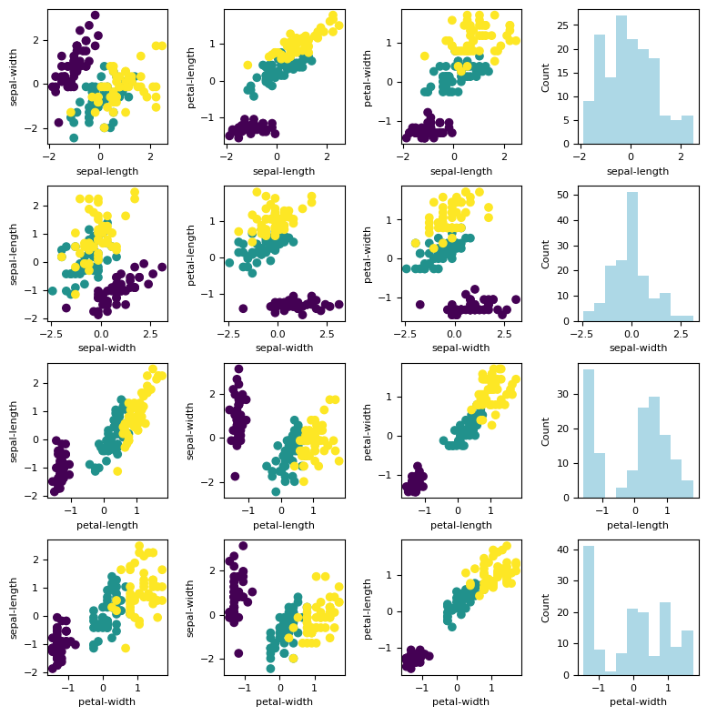
Standardization
Definition:
means  = np.mean(X, axis=0)
stdevs = np.std(X, axis=0)

X_std = (X - means) / stdevs
Let us plot the standardized dataset.
%matplotlib inline

fig, ax = plt.subplots(nrows=n_features, ncols=n_features, figsize= (n_features*2, n_features*2))
fig.tight_layout(pad=2.0)

names = feature_names

for i in range(n_features):
    J = np.arange(n_features)
    J = np.delete(J, i)
    for k, j in enumerate(J):
        ax[i, k].scatter(X_std[:, i], X_std[:, j], c = y)
        ax[i, k].set_xlabel(names[i])
        ax[i, k].set_ylabel(names[j])

for i in range(n_features):
    ax[i, -1].hist(X_std[:, i], color = 'lightblue')
    ax[i, -1].set_ylabel('Count')
    ax[i, -1].set_xlabel(names[i])
Covariance Matrix
Defintion:
where:
and
cov_mat = np.cov(X_std.T) # square symmetric, positive semi-definite
cov_mat
array([[ 1.007, -0.11 ,  0.878,  0.823],
       [-0.11 ,  1.007, -0.423, -0.359],
       [ 0.878, -0.423,  1.007,  0.969],
       [ 0.823, -0.359,  0.969,  1.007]])
Singular Value Decompostion
Defintion:
For square symmetric positive semi-definite matrix (such as covariance matrix), the eigenvalues and \(\operatorname{diag}(\Sigma)\) are exactly the same and \(U\) is the Eigen-vector matrix.
U, S, V = np.linalg.svd(cov_mat)
eig_vals = S
eig_vecs = U

print ("Eigen values (lambda):")
print(S)
print()
print("Corresponding Eigen-vector matrix (U):")
print(U)
Eigen values (lambda):
[2.93  0.927 0.148 0.021]

Corresponding Eigen-vector matrix (U):
[[-0.522 -0.372  0.721  0.262]
 [ 0.263 -0.926 -0.242 -0.124]
 [-0.581 -0.021 -0.141 -0.801]
 [-0.566 -0.065 -0.634  0.524]]
Correct the Eigen-vector Matrix
This section is actually optional. This step is necessary if we want to keep our results identical to PCA from scikit-learn.
Correct the Eigen matrix such that:
for each column, find the largest absolute value
if the largest absolute value comes from a negative value, make it positive by multiplying the entire column with -1
# Adjusting the eigenvectors (loadings) that are largest in absolute value to be positive
max_abs_idx = np.argmax(np.abs(eig_vecs), axis=0)
signs = np.sign(eig_vecs[max_abs_idx, range(eig_vecs.shape[0])])
eig_vecs_ = eig_vecs*signs[np.newaxis,:]

print(eig_vals)
print()
print(eig_vecs_)
[2.93  0.927 0.148 0.021]

[[ 0.522  0.372  0.721 -0.262]
 [-0.263  0.926 -0.242  0.124]
 [ 0.581  0.021 -0.141  0.801]
 [ 0.566  0.065 -0.634 -0.524]]
Select the Axis Components
Let us introdue \(W\) as the new axis components where: $\( W \in (U_{i,j})_{1\leq j<k}\)$
As an example, let us take \(k=2\).
# Select top k eigenvectors
k = 2
W = eig_vecs_[:, :k] # Projection matrix
print(W)
print(W.shape)
[[ 0.522  0.372]
 [-0.263  0.926]
 [ 0.581  0.021]
 [ 0.566  0.065]]
(4, 2)
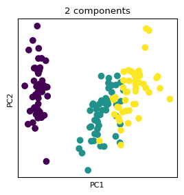
Project the Dataset to the New Axis Components
Let us introduce \(X_\text{proj}\) to represent the transformed dataset:
X_proj = X_std.dot(W)
print(X_proj.shape)
(150, 2)
%matplotlib inline

fig, ax = plt.subplots(figsize=(3,3))

ax.scatter(X_proj[:, 0], X_proj[:, 1], c = y)
ax.set_xlabel('PC1'); plt.xticks([])
ax.set_ylabel('PC2'); plt.yticks([])
ax.set_title('2 components');
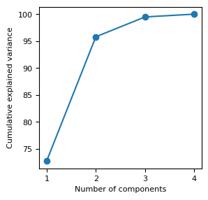
Explained Variance
The optimal value for k can be tuned by investigating the explained variance.
The explained variance tells us how much information (variance) can be attributed to each of the principal components.
where: \(r<= m\)
%matplotlib inline

eig_vals_total = sum(eig_vals)
explained_variance = [(i / eig_vals_total)*100 for i in eig_vals]
explained_variance = np.round(explained_variance, 2)
cum_explained_variance = np.cumsum(explained_variance)

print('Explained variance: {}'.format(explained_variance))
print('Cumulative explained variance: {}'.format(cum_explained_variance))

fig, ax = plt.subplots(figsize= (3, 3))

ax.plot(np.arange(1,n_features+1), cum_explained_variance, '-o')
ax.set_xticks(np.arange(1,n_features+1))
ax.set_xlabel('Number of components')
ax.set_ylabel('Cumulative explained variance');
Explained variance: [72.77 23.03  3.68  0.52]
Cumulative explained variance: [ 72.77  95.8   99.48 100.  ]
[OPTIONAL] Comparison to scikit-learn
from sklearn.decomposition import PCA

pca = PCA(n_components=2)
pca.fit_transform(X_std)

print('by sklearn:')
print(pca.components_.transpose())

print('ours:')
print(W)
by sklearn:
[[ 0.522  0.372]
 [-0.263  0.926]
 [ 0.581  0.021]
 [ 0.566  0.065]]
ours:
[[ 0.522  0.372]
 [-0.263  0.926]
 [ 0.581  0.021]
 [ 0.566  0.065]]
Breast Cancer Wisconsin
In this section, we are going to exactly repeat the process but with different dataset. This time we are going to use the “Breast Cancer Winsconsin” dataset. The dataset can be found in this link.
Load the Dataset
data = np.loadtxt("./datasets/breast_cancer/wdbc.data", delimiter=",", dtype=str)
X = np.float32(data[:, 2:12])  # 10 dimensions

# Diagnosis (M = malignant, B = benign)
y = np.zeros(X.shape[0], dtype=np.int32)
y[np.where(data[:,1]=='M')] = 1
y[np.where(data[:,1]=='B')] = 0

n_features = X.shape[1]
feature_names = ['#'+str(k) for k in range(n_features)]

print("Dimension numbers :", X.shape[1])
print("Number of data    :", X.shape[0])
print("Labels            :", np.unique(y))
Dimension numbers : 10
Number of data    : 569
Labels            : [0 1]
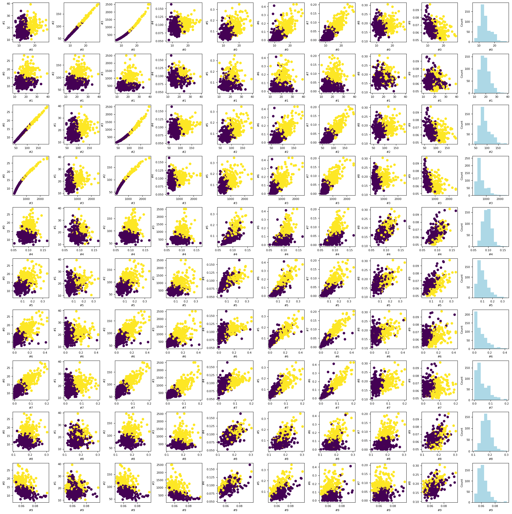
%matplotlib inline

fig, ax = plt.subplots(nrows=n_features, ncols=n_features, figsize= (n_features*2, n_features*2))
fig.tight_layout(pad=2.0)

names = feature_names

for i in range(n_features):
    J = np.arange(n_features)
    J = np.delete(J, i)
    for k, j in enumerate(J):
        ax[i, k].scatter(X[:, i], X[:, j], c = y)
        ax[i, k].set_xlabel(names[i])
        ax[i, k].set_ylabel(names[j])

for i in range(n_features):
    ax[i, -1].hist(X[:, i], color = 'lightblue')
    ax[i, -1].set_ylabel('Count')
    ax[i, -1].set_xlabel(names[i])
Standardization
means  = np.mean(X, axis=0)
stdevs = np.std(X, axis=0)

X_std = (X - means) / stdevs
%matplotlib inline

fig, ax = plt.subplots(nrows=n_features, ncols=n_features, figsize= (n_features*2, n_features*2))
fig.tight_layout(pad=2.0)

names = feature_names

for i in range(n_features):
    J = np.arange(n_features)
    J = np.delete(J, i)
    for k, j in enumerate(J):
        ax[i, k].scatter(X_std[:, i], X_std[:, j], c = y)
        ax[i, k].set_xlabel(names[i])
        ax[i, k].set_ylabel(names[j])

for i in range(n_features):
    ax[i, -1].hist(X_std[:, i], color = 'lightblue')
    ax[i, -1].set_ylabel('Count')
    ax[i, -1].set_xlabel(names[i])

Covariance Matrix
cov_mat = np.cov(X_std.T) # square symmetric, positive semi-definite
print(cov_mat)
[[ 1.002  0.324  1.     0.989  0.171  0.507  0.678  0.824  0.148 -0.312]
 [ 0.324  1.002  0.33   0.322 -0.023  0.237  0.303  0.294  0.072 -0.077]
 [ 1.     0.33   1.002  0.988  0.208  0.558  0.717  0.852  0.183 -0.262]
 [ 0.989  0.322  0.988  1.002  0.177  0.499  0.687  0.825  0.152 -0.284]
 [ 0.171 -0.023  0.208  0.177  1.002  0.66   0.523  0.555  0.559  0.586]
 [ 0.507  0.237  0.558  0.499  0.66   1.002  0.885  0.833  0.604  0.566]
 [ 0.678  0.303  0.717  0.687  0.523  0.885  1.002  0.923  0.502  0.337]
 [ 0.824  0.294  0.852  0.825  0.555  0.833  0.923  1.002  0.463  0.167]
 [ 0.148  0.072  0.183  0.152  0.559  0.604  0.502  0.463  1.002  0.481]
 [-0.312 -0.077 -0.262 -0.284  0.586  0.566  0.337  0.167  0.481  1.002]]
Singular Value Decomposition
U, S, V = np.linalg.svd(cov_mat)
eig_vals = S
eig_vecs = U

print ("Eigen values (lambda):")
print(S)
print()
print("Corresponding Eigen-vector matrix (U):")
print(U)
Eigen values (lambda):
[5.488 2.523 0.882 0.5   0.373 0.124 0.08  0.035 0.011 0.   ]

Corresponding Eigen-vector matrix (U):
[[-0.364  0.314 -0.124 -0.03   0.031  0.264  0.044 -0.085 -0.474  0.669]
 [-0.154  0.147  0.951 -0.009  0.22   0.032 -0.021  0.007 -0.004 -0.   ]
 [-0.376  0.285 -0.114 -0.013  0.006  0.238  0.083 -0.089 -0.38  -0.74 ]
 [-0.364  0.305 -0.123 -0.013  0.019  0.332 -0.261 -0.145  0.747  0.032]
 [-0.232 -0.402 -0.167  0.108  0.844 -0.062 -0.011 -0.171 -0.006 -0.004]
 [-0.364 -0.266  0.058  0.186 -0.24  -0.005  0.804 -0.064  0.219  0.053]
 [-0.396 -0.104  0.041  0.167 -0.313 -0.601 -0.367 -0.45  -0.081  0.01 ]
 [-0.418 -0.007 -0.069  0.073  0.009 -0.266 -0.141  0.851  0.022  0.004]
 [-0.215 -0.368  0.037 -0.893 -0.113  0.062 -0.048 -0.016 -0.009 -0.001]
 [-0.072 -0.572  0.114  0.349 -0.265  0.568 -0.345  0.065 -0.13  -0.007]]
Correct the Eigen-vector Matrix
# Adjusting the eigenvectors (loadings) that are largest in absolute value to be positive
max_abs_idx = np.argmax(np.abs(eig_vecs), axis=0)
signs = np.sign(eig_vecs[max_abs_idx, range(eig_vecs.shape[0])])
eig_vecs_ = eig_vecs*signs[np.newaxis,:]

print(eig_vals)
print()
print(eig_vecs_)
[5.488 2.523 0.882 0.5   0.373 0.124 0.08  0.035 0.011 0.   ]

[[ 0.364 -0.314 -0.124  0.03   0.031 -0.264  0.044 -0.085 -0.474 -0.669]
 [ 0.154 -0.147  0.951  0.009  0.22  -0.032 -0.021  0.007 -0.004  0.   ]
 [ 0.376 -0.285 -0.114  0.013  0.006 -0.238  0.083 -0.089 -0.38   0.74 ]
 [ 0.364 -0.305 -0.123  0.013  0.019 -0.332 -0.261 -0.145  0.747 -0.032]
 [ 0.232  0.402 -0.167 -0.108  0.844  0.062 -0.011 -0.171 -0.006  0.004]
 [ 0.364  0.266  0.058 -0.186 -0.24   0.005  0.804 -0.064  0.219 -0.053]
 [ 0.396  0.104  0.041 -0.167 -0.313  0.601 -0.367 -0.45  -0.081 -0.01 ]
 [ 0.418  0.007 -0.069 -0.073  0.009  0.266 -0.141  0.851  0.022 -0.004]
 [ 0.215  0.368  0.037  0.893 -0.113 -0.062 -0.048 -0.016 -0.009  0.001]
 [ 0.072  0.572  0.114 -0.349 -0.265 -0.568 -0.345  0.065 -0.13   0.007]]
Select the Axis Components
# Select top k eigenvectors
k = 3
W = eig_vecs_[:, :k] # Projection matrix
print(W)
print(W.shape)
[[ 0.364 -0.314 -0.124]
 [ 0.154 -0.147  0.951]
 [ 0.376 -0.285 -0.114]
 [ 0.364 -0.305 -0.123]
 [ 0.232  0.402 -0.167]
 [ 0.364  0.266  0.058]
 [ 0.396  0.104  0.041]
 [ 0.418  0.007 -0.069]
 [ 0.215  0.368  0.037]
 [ 0.072  0.572  0.114]]
(10, 3)
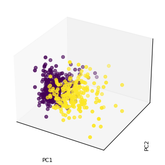
Project the Dataset to the New Axis Components
X_proj = X_std.dot(W)
print(X_proj.shape)
(569, 3)
%matplotlib inline

fig = plt.figure(figsize=(4,4));
ax = fig.add_subplot(projection='3d');

ax.scatter(X_proj[:, 0], X_proj[:, 1],  X_proj[:, 2], c = y);

ax.set_xlabel('PC1');
ax.set_xticks([]);
ax.set_ylabel('PC2', rotation=90);
ax.set_yticks([]);
ax.set_zlabel('PC3', rotation=90);
ax.set_zticks([]);
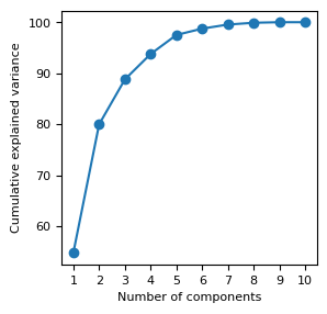
Explained Variance
%matplotlib inline

eig_vals_total = sum(eig_vals)
explained_variance = [(i / eig_vals_total)*100 for i in eig_vals]
explained_variance = np.round(explained_variance, 2)
cum_explained_variance = np.cumsum(explained_variance)

print('Explained variance: {}'.format(explained_variance))
print('Cumulative explained variance: {}'.format(cum_explained_variance))

fig, ax = plt.subplots(figsize= (3, 3))

ax.plot(np.arange(1,n_features+1), cum_explained_variance, '-o')
ax.set_xticks(np.arange(1,n_features+1))
ax.set_xlabel('Number of components')
ax.set_ylabel('Cumulative explained variance');
Explained variance: [54.79 25.19  8.81  4.99  3.73  1.24  0.8   0.35  0.11  0.  ]
Cumulative explained variance: [ 54.79  79.98  88.79  93.78  97.51  98.75  99.55  99.9  100.01 100.01]
[OPTIONAL] Comparison to scikit-learn
from sklearn.decomposition import PCA

pca = PCA(n_components=3)
pca.fit_transform(X_std)

print('by sklearn:')
print(pca.components_.transpose())

print('ours:')
print(W)
by sklearn:
[[ 0.364 -0.314 -0.124]
 [ 0.154 -0.147  0.951]
 [ 0.376 -0.285 -0.114]
 [ 0.364 -0.305 -0.123]
 [ 0.232  0.402 -0.167]
 [ 0.364  0.266  0.058]
 [ 0.396  0.104  0.041]
 [ 0.418  0.007 -0.069]
 [ 0.215  0.368  0.037]
 [ 0.072  0.572  0.114]]
ours:
[[ 0.364 -0.314 -0.124]
 [ 0.154 -0.147  0.951]
 [ 0.376 -0.285 -0.114]
 [ 0.364 -0.305 -0.123]
 [ 0.232  0.402 -0.167]
 [ 0.364  0.266  0.058]
 [ 0.396  0.104  0.041]
 [ 0.418  0.007 -0.069]
 [ 0.215  0.368  0.037]
 [ 0.072  0.572  0.114]]