Convolutional Layers

Preparations

import numpy as np
from scipy.optimize import minimize
import matplotlib.pyplot as plt
from matplotlib import image

plt.rcParams.update({
    "text.usetex": True,
    "font.family": "sans-serif",
    "font.size": 10,
})

from utils import *

np.set_printoptions(precision=5, suppress=True)

Single Image Convolution

A convolution is done by multiplying a pixel’s and its neighboring pixels color value by a matrix (kernel matrix).

Here, we implement a convolution function for a single image. The implemenation is as follows, where:

• img_in is the image as a 2D matrix

• kernel is the filter kernel matrix

• S is the stride number

def convolve(img_in, kernel, S):
    F, _ = kernel.shape
    nr, nc, = img_in.shape

    R = np.arange(0, nr - (F - S), S)
    C = np.arange(0, nc - (F - S), S)
    
    img_out = np.zeros([len(R), len(C)])

    for i, r in enumerate(R):
        for j, c in enumerate(C):
            img_out[i, j] = np.sum(kernel * img_in[r:r+F, c:c+F])

    return img_out

Typically, when s = 1, the dimension should not change. This is possible if the image has been previously padded. For a 3 x 3 filter matrix, we need 1 layer of padding. For a 5 x 5 filter matrix, we will need two layes of padding. However, if the filter dimensions are even numbers, we will not be able to apply uniform padding. Check this material for more infomation.

Single Image Pooling

Pooling is a downsampling technique used in convolutional neural networks (CNNs) to reduce spatial dimensions of feature maps while preserving important features. It achieves this by selecting the maximum/mean value within each small, overlapping region (or “window”) of the feature map.

def maxpool(img_in, F, S):
    nr, nc, = img_in.shape

    R = np.arange(0, nr - (F - S), S)
    C = np.arange(0, nc - (F - S), S)
    
    img_out = np.zeros([len(R), len(C)])

    for i, r in enumerate(R):
        for j, c in enumerate(C):
            img_out[i, j] = np.max(img_in[r:r+F, c:c+F])

    return img_out

def meanpool(img_in, F, S):
    nr, nc, = img_in.shape

    R = np.arange(0, nr - (F - S), S)
    C = np.arange(0, nc - (F - S), S)
    
    img_out = np.zeros([len(R), len(C)])

    for i, r in enumerate(R):
        for j, c in enumerate(C):
            img_out[i, j] = np.mean(img_in[r:r+F, c:c+F])

    return img_out

Single Image Normalization

This is a simple min-max normalization. This process causes the pixel values to range from 0 to 1.

def normalize(img_in):
    min_val = np.min(img_in)
    max_val = np.max(img_in)
    return (img_in - min_val) / (max_val - min_val)

Batch Convolution

• I: number of the input images, the dimensions of all images are W x H

• O: number of output images

• I x O: number of the convolution filters (kernels)

• F x F: dimension of the kernels

• S: stride length

• P: number of padding layers

• The dimension of the output images are W2 x H2, where: W2 = (W - F + 2 * P) / S + 1) and H2 = (H - F + 2 * P) / S + 1)

def batch_convolve(input3d, filter4d, bias1d, P, S=1):
    # Volumetric matrix is addressed by using 3 indices: [first index, second index, third index]
    # Depth is represented first index
    H, W, I = input3d.shape;
    F, _, _, O = filter4d.shape;
    
    # Do ZERO padding
    input3d = np.pad(input3d, ((P, P), (P, P), (0, 0)), 'constant', constant_values=((0, 0), (0, 0),(0, 0)))

    W2 = np.int32((W - F + 2 * P) / S + 1)
    H2 = np.int32((H - F + 2 * P) / S + 1)
    O = np.int32(O)  
    I = np.int32(I)

    output3d = np.zeros((W2, H2, O), dtype=np.float32)

    for o in range(O):
        output3d[:, :, o] = output3d[:, :, o] + bias1d[o]
        for i in range(I):
            input = input3d[:, :, i]
            output3d[:, :, o] = output3d[:, :, o] + convolve(input, kernel=filter4d[:, :, i, o], S=S)

    return output3d

Batch Pooling

Batch pooling involves:

• D images with a dimension of W x H

• a pooling filter of F x F

• a stride length of S

def batch_maxpool(input3d, F, S):
    H, W, D = input3d.shape;

    W2 = np.int32((W - F) / S + 1)
    H2 = np.int32((H - F) / S + 1)
    D2 = np.int32(D)

    output3d = np.zeros((W2, H2, D2), dtype=np.float32)

    for d2 in range(D2):
        input = input3d[:, :, d2]
        output3d[:, :, d2] = maxpool(input, F, S)

    return output3d

def batch_meanpool(input3d, F, S):
    H, W, D = input3d.shape;

    W2 = np.int32((W - F) / S + 1)
    H2 = np.int32((H - F) / S + 1)
    D2 = np.int32(D)

    output3d = np.zeros((W2, H2, D2), dtype=np.float32)

    for d2 in range(D2):
        input = input3d[:, :, d2]
        output3d[:, :, d2] = meanpool(input, F, S)

    return output3d

Batch Normalization

def batch_normalization(input3d):
    H, W, D = input3d.shape;
    output3d = np.zeros((W, H, D), dtype=np.float32)

    for d in range(D):
        output3d[:, :, d] = normalize(input3d[:, :, d])

    return output3d

Activations

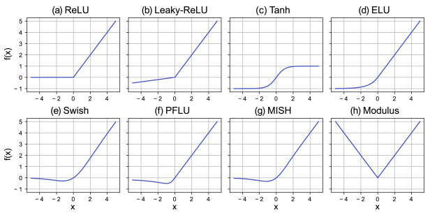
def ReLU(input3d):
    return (np.maximum(0, input3d))

def LeakyReLU(input3d):
    return (np.maximum(0.1*input3d, input3d))

---

Demonstrations

1. Batch Convolution of an Image

For the demonstration, we will load a colored image (3 channels).

%matplotlib inline

baboon = np.int32(image.imread('./baboon.png') * 255.0)
print("image dimension:", baboon.shape)

plt.imshow(baboon)
plt.show()

image dimension: (512, 512, 3)

For the sake of clarity, let us plot the loaded image as three different grayscale images

%matplotlib inline
for i in range(3):
    plt.subplot(1, 3, i+1)
    plt.imshow(baboon[:, :, i], cmap='Greys')
    plt.axis('off')

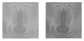
Let’s apply (3 x 3 x 3 x 2) arbitrary filters:

• filter kernel dimesion: 3 x 3

• number of inputs: 3

• number of outputs: 2

F = np.zeros((3, 3, 3, 2))

F[:,:, 0, 0] = np.array([[0.0625, 0.125, 0.0625],
                         [0.125, 0.25, 0.125],
                         [0.0625, 0.125, 0.0625]])

F[:,:, 0, 1] = np.array([[-2, -1,  0],
                         [-1,  1,  1],
                         [ 0,  1,  2]])

F[:,:, 1, 0] = np.array([[-1, -1, -1],
                         [-1, 8, -1],
                         [-1, -1, -1]])

F[:,:, 1, 1] = np.array([[1, 0, -1],
                         [2, 0, -2],
                         [1, 0, -1]])

F[:,:, 2, 0] = np.array([[-1, -1, -1],
                         [-1, 8, -1],
                         [-1, -1, -1]])

F[:,:, 2, 1] = np.array([[-1, 0, 1],
                         [-2, 0, 2],
                         [-1, 0, 1]])


bias = np.zeros(2)

output = batch_convolve(baboon, F, bias, 1)
output = batch_meanpool(output, 2, 2)
output = batch_normalization(output)
output = ReLU(output)

for i in range(output.shape[2]):
    plt.subplot(1, 3, i+1)
    # Rescale the weights to be between 0 and 255
    plt.imshow(output[:,:, i]*255, cmap='Greys')
    plt.axis('off')

---

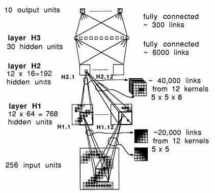
2. LeNet-1

The following picture is the LeNet-1 layer architecture diagram.

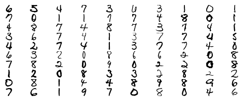
First, we load the USPS datasets. There are two sets of data: training data and testing data.

import h5py
with h5py.File("./datasets/usps/usps.h5", 'r') as hf:
    x_train = hf.get("train").get('data')[:].reshape(-1, 16, 16) * 255.0
    y_train = np.int32(hf.get("train").get('target')[:]) 

    x_test = hf.get("test").get('data')[:].reshape(-1, 16, 16) * 255.0
    y_test = np.int32(hf.get("test").get('target')[:]) 

print("Training data:")
print("Dimension numbers :", x_train.shape[1] * x_train.shape[2])
print("Number of data    :", x_train.shape[0])

print("\nTesting data:")
print("Dimension numbers :", x_test.shape[1] * x_test.shape[2])
print("Number of data    :", x_test.shape[0])

Training data:
Dimension numbers : 256
Number of data    : 7291

Testing data:
Dimension numbers : 256
Number of data    : 2007

# Peforming reshaping operation
x_train = x_train.reshape(x_train.shape[0], 16, 16, 1)
x_test = x_test.reshape(x_test.shape[0], 16, 16, 1)

for i in range(100):
    X = x_train[i,:,:]
    plt.subplot(20, 10, i + 1)
    plt.imshow(X.astype('uint8'), cmap='Greys')
    plt.axis('off')

Next, we also load all weight matrices and bias vectors from the previously trained network as found in lenet1.ipynb.

w1  = np.load('./datasets/usps/weight-1.npy')  # weight
w2  = np.load('./datasets/usps/weight-2.npy')  # bias
w3  = np.load('./datasets/usps/weight-3.npy')  # weight
w4  = np.load('./datasets/usps/weight-4.npy')  # bias
w5  = np.load('./datasets/usps/weight-5.npy')  # weight
w6  = np.load('./datasets/usps/weight-6.npy')  # bias
w7  = np.load('./datasets/usps/weight-7.npy')  # weight
w8  = np.load('./datasets/usps/weight-8.npy')  # bias
w9  = np.load('./datasets/usps/weight-9.npy')  # weight
w10 = np.load('./datasets/usps/weight-10.npy') # bias

We then tranlsate the layer architecture diagram into actual codes.

The sequential order of the CNN is as follows:

input --> C1 --> reLU --> M1 --> C2 --> ReLU --> M2 --> FCN

where C and M are convolutional and max-pooling layers, respectively. FCN is a fully-connected network layer.

y_predict = []
for k in range(x_test.shape[0]):
    # C1
    output1 = batch_convolve(x_test[k].reshape(16, 16, 1), w1, w2, 2)
    output2 = ReLU(output1)
    # M1
    output3 = batch_maxpool(output2, 2, 2)
    # C2
    output4 = batch_convolve(output3, w3, w4, 2)
    output5 = ReLU(output4)
    # M2
    output6 = batch_maxpool(output5, 2, 2)

    # FCN
    output7 = output6.flatten()
    output7 = output7.reshape(1, 192)
    y1 = output7 @ w5 + w6
    y2 = np.maximum(0, y1)
    y3 = y2 @ w7 + w8
    y4 = np.maximum(0, y3)
    y5 = y4 @ w9 + w10
    y_predict.append(np.argmax(y5))

y_predict = np.array(y_predict)

Do predictions by using the loaded weights and check the accuracy.

# Predict on the validation set
val_acc = (y_predict == y_test).mean()
print('Validation accuracy : ', val_acc)

Validation accuracy :  0.953662182361734